Department of Electrical Engineering and Computer Science
1. Introduction
Many network simulators, such as NS2, Openet, Qualnet, etc., are widely
available. We'll use NS2 for this project. NS2 is a discrete event simulator
written in C++, with an OTcl interpreter shell as the user interface that
allows the input model files (Tcl scripts) to be executed. Most network
elements in the NS2 simulator are developed as classes, in object-oriented
fashion. The simulator supports a class hierarchy in C++, and a very
similar class hierarchy in OTcl. The root of this class hierarchy is the
TclObject in OTcl. Users create new simulator objects through the OTcl
interpreter, and then these objects are mirrored by corresponding objects
in the class hierarchy in C++. NS2 provides substantial support for simulation
of TCP, routing algorithms, queueing algorithms, and multicast protocols
over wired and wireless (local and satellite) networks, etc. It is freely
distributed, and all source code is available.
Developing new networking protocols and creating simulation scripts
are complex tasks, which requires understanding of the NS2 class hierarchy,
C++, and Tcl programming. However, in this project, you only need to design
and run simulations in Tcl scripts using the simulator objects without
changing NS2 core components such as the class hierarchy, event schedulers,
and other network building blocks. You'll focus on simulation and analysis
of some different windowing mechanisms and TCP variants. You should
put all your results in the files with given names. For your report, you
do not need to rewrite the assumptions given in this document, but should
provide any information not already given to you. This project has to be
done individually but not in groups.
2. Objectives
Following are a few useful NS2 tutorial documents or web sites (you'll
find valuable information on NS2 as well as some useful simulation examples):
In EECS department, NS2 2.1b9a has already been installed
under directory "/share/instsww/pkg/ns-allinone-2.1b9a/bin" (http://inst.eecs.berkeley.edu/cgi-bin/pub.cgi?file=ns.help).
Although it is not the latest version (NS2
2.27, released Jan 18, 2004), it is still good for this project.
Several other software tools are very useful for running the ns simulations
scripts: Otcl, Nam, Gnuplot, XGraph, Awk, and Perl. The script itself is
in Otcl, which is an object-oriented version of Tcl, a well-known scripting
language. Nam is a Tcl/Tk based animation tool for visualizing network
simulation traces and real world packet traces. Gnuplot and XGraph are
general plotting tools, and we use them to plot simulation results. Awk
and Perl are text-processing languages and we use them to parse the trace
files for further analysis. If you want more information about these software
tools, please go to class web site of Project 2.
You may also want to install NS2 and related software package on your
LINUX machine. The all-in-one
NS2 package can be downloaded from NS2 web site (http://www.isi.edu/nsnam/ns/ns-build.html).
There is a Windows version of NS2. However, it doesn't work as well as
the UNIX/LINUX version, so use it at your own risk.
4. Task Description
You are given a sample file (task1_sample.tcl) to simulate the above-mentioned
network. Run the simulation for 5 seconds by typing "ns task1_sample.tcl",
and then we obtain an output trace file, task1_out.nam. You need to understand
the trace format and be able to extract meaningful performance metrics
from such files by using Awk, Perl, etc. Take a look at "task1_out.nam".
Ignore entries with -t *; these entries are used by nam to visualize the
network topology. The rest of the entries look like:
In this command, "$1", "$7", "$17", and "$9" mean the 1st (event type),
7th (destination node), 17th (flow identifier) , and 9th (packet type)
columns of each line in file "task1_out.nam". "a" is an Awk variable that
is used to calculate the total bytes. Awk scans the input file "task1_out.nam"
line by line, and parses the line column by column.
# create links between the nodes
# set the display layout of nodes and links for nam
# define different colors for nam data flows
# monitor the queue for the link between node 2 and node 3
# window_ * (packetsize_ + 40) / RTT
# create a TCP sink agent and attach it to node node4
# connect both agents
# create an FTP source "application";
# window_ * (packetsize_ + 40) / RTT # create a TCP sink agent and attach it to node node4 # connect both agents # create an FTP source "application"; #Define a 'finish' procedure
# close the nam trace
file
# execute nam on the
trace file
# call the finish procedure after 6 seconds of simulation time
# run the simulation
(b) (task1_b.tcl) Revise the sample code "task1_sample.tcl"
so that the window size of the second TCP flow (tcp2) changes from 25
to 5. In the real world, such a change might occur if one were to
switch from browing the internet with one's home computer to browing on
one's cell phone. Because the resources are much more limited, the
window size drops dramatically. Use the given Awk scripts to compute
the total traffic of both flows. How does the packet rate loss change?
Which flow uses more bandwidth in the bottleneck from node 3 to node 4?
What is the reason? (c) (task1_c.tcl)
Revise the sample code "task1_sample.tcl" so that the window size of both the TCP flows are set to 5. Use the given Awk scripts to compute the total traffic of both flows. Give the total bytes of traffic for each flow. How does the packet loss rate change? Do both flows receive a "fair share" of the available bandwidth of the bottleneck link? What is the reason? Present your results for a-c in a table. (d)
(task1_d.tcl, task1_d_total.awk) Now node 5 is added to the network configuration in part c). It is connected to node 3. The link between node 5 and node 3 has a speed of 2 Mbps and a propagation delay of 10 ms. The new network topology is shown in Figure 2. One more TCP/FTP flow with a window size of 5 is generated from node 5 to node 4. Revise the sample code "task1_sample.tcl" for the new network, and run the simulation. Revise the sample Awk command in file "task1_total.awk" to compute the total bytes of TCP from each flow. Give the total bytes of TCP for each flow. Do all the TCP flows receive a fair "share" of the bandwidth? Why or why not? Task 2: Different Flavors of TCP
To get the tcl scripts and binary needed for task 2, download the following file: task2.tar
Task 2: Different Flavors of TCP The Internet suffered from
congestion collapse in the late 80's. As a result, several congestion control
algorithms were proposed and implemented to prevent the TCP senders from
overwhelming the resources of the network. In 1988, TCP Tahoe was introduced
with three congestion control algorithms: slow start, additive
increase/multiplicative decrease (AIMD), and fast retransmit. Since then, many
modifications have been made to TCP and several different versions of TCP have been
implemented. TCP Reno revises TCP Tahoe by modifying the fast retransmit to
include fast recovery. Another conservative extension of TCP Reno is TCP SACK,
which adds Selective Acknowledgment to TCP. In this project, you'll study these
three variants of TCP protocol: Tahoe, Reno, and SACK. In NS2, TCP Tahoe is the default implementation and such a
sender agent is called Agent/TCP. Other TCP sender agents are obtained by
adding the TCP variant names to the base name, for example,
Agent/TCP/Reno, Agent/TCP/Sack1. Except
TCP SACK, you only need to change the sender agent, and these TCP variants use
the same receiver agent, Agent/TCPSink. On the other hand, for TCP SACK, you
will also need to change the sink agent to Agent/TCPSink/Sack1.
Project 2 Specification v 1.0
University of California, Berkeley
In a complex, dynamic, expensive, and large-scale system like the Internet,
analytic solutions are usually not known or are only approximately known.
Due to many practical reasons such as cost, risk, and controllability,
etc., real experiments on the actual network system may not be preferred.
Network simulators attempt to represent real world networks by modeling
key elements of the real system and incorporating most of its salient features.
Furthermore, it is not too complex for us to understand and experiment
with them. The models and their operations enable us to predict the behavior
of actual systems at low cost under different configurations of interest
and over long period. Although network simulators are not perfect, they
are usually accurate enough to give us a meaningful insight into how the
network is working, and how its operation can be optimized.
3. Using NS2
To run NS2, we need to add the appropriate directory to PATH environment
variable.
source /share/instsww/pkg/ns-allinone-2.1b9a/ns.cshrc
ns task1_sample.tcl
nam task1_out.nam
The GUI interface is shown below. You can press the play button to begin
the animation.
Task 1: Bandwidth Share of TCP flows with different Window Sizes
Consider a network with 4 nodes, as shown in Figure 1. The link between
node 3 and node 4 has a speed of 1 Mbps. All other links have a speed
of
2 Mbps. All links have a propagation delay of 10 ms and a Drop Tail
buffer.
There is a TCP/FTP flow from node 1 to node 4 and from node 2 to node
4. Both start at 0.1 second, and end
at 5 seconds. The packet length for both flows is 1000 Bytes, and they
both have a window size of 25 packets. The queue buffer size for the
link from
node 3 to node 4 is 4 packets. There is no other traffic in the network
other than that described above.

Figure 1
The fields in the trace file are: type of the event, simulation time when
the event occurred, source and destination nodes, packet type (protocol,
action or traffic source), packet size, color type, packet ID, flow identifier,
source and destination addresses, sequence number, and packet id. Note
that the internal identifier numbers for node 1, node 2, node 3, and node
4 are 0, 1, 2, and 3, respectively. The event type "+", "-", "r", and "d"
represent enqueue operations, dequeue operations, receive events, and drop
events, respectively. Although we have a strong preference for you to use
Awk to answer the following question, you can use other languages such
as perl to compute these metrics if you prefer, but you are on your own
(sample code for other languages is not available).
awk '$1== "r" && $7==3 && $17==1 && $9=="tcp"
{a += $11} END {print a}' task1_out.nam
awk '$1=="r" && $7==3 && $17==2 && $9=="tcp"
{b += $11} END {print b}' task1_out.nam
awk '$1=="d" {c += $11} END {print c}' task1_out.nam
awk '{if ($1== "r" && $7==3 && $17==1 &&
$9=="tcp") {a += $11} else if ($1== "r" && $7==3 &&
$17==2 && $9=="tcp") {b += $11} else if ($1=="d") {c += $11}} END {printf (" tcp1:\t%d\n tcp2:\t%d
\n total:\t%d\n tcp1 ratio:\t%.4f \n tcp2 ratio:\t%.4f\n Dropped Packets:\t%d\n ", a, b, a+b, a/(a+b),
b/(a+b), c)}' task1_out.nam
Let's take a look at the Tcl scripts in "task1_sample.tcl", and
go through the sequence of required steps to set up and solve a simulation
problem:
# create a simulator object
set ns [new Simulator]# create four nodes
set node1 [$ns node]
set node2 [$ns node]
set node3 [$ns node]
set node4 [$ns node]
$ns duplex-link $node1 $node3 2Mb 10ms DropTail
$ns duplex-link $node2 $node3 2Mb 10ms DropTail
$ns duplex-link $node3 $node4 1Mb 10ms DropTail
$ns queue-limit $node3 $node4 4
$ns duplex-link-op $node1 $node3 orient right-down
$ns duplex-link-op $node2 $node3 orient right-up
$ns duplex-link-op $node3 $node4 orient right
$ns color 0 Green
$ns color 1 Blue
$ns color 2 Red
$ns color 3 Yellow
$ns duplex-link-op $node3 $node4 queuePos 0.5
# First TCP traffic source
# create a TCP agent and attach it to node node1
set tcp1 [new Agent/TCP]
$ns attach-agent $node1 $tcp1
$tcp1 set fid_ 1
$tcp1 set class_ 1
$tcp set window_ 25
$tcp set packetSize_ $packetSize
set sink [new Agent/TCPSink]
$ns attach-agent $node4 $sink
$ns connect $tcp1 $sink
set ftp1 [new Application/FTP]
$ftp1 attach-agent $tcp1
# create a TCP agent and attach it to node node1
set tcp2 [new Agent/TCP]
$ns attach-agent $node2 $tcp2
$tcp2 set fid_ 2
$tcp2 set class_ 2
$tcp2 set window_ 25
$tcp2 set packetSize_ $packetSize
set sink2 [new Agent/TCPSink]
$ns attach-agent $node4 $sink2
$ns connect $tcp2 $sink2
set ftp2 [new Application/FTP]
$ftp2 attach-agent $tcp2
# open the nam trace file
set nam_trace_fd [open tcp_tahoe.nam w]
$ns namtrace-all $nam_trace_fd
set trace_fd [open tcp_tahoe.tr w]
proc finish {} {
global ns nam_trace_fd
trace_fd
$ns flush-trace
close $nam_trace_fd
exit 0
}
# schedule events for all the flows
$ns at 0.1 "$ftp1 start"
$ns at 0.1 "$ftp2 start"
$ns at 5.0 "$ftp2 stop"
$ns at 5.0 "$ftp1 stop"
$ns at 6 "finish"
$ns run
(a) (task1.pdf) Based on the execution results of previous Awk
commands, what is the packet loss rate of the two TCP flows? What is
the ratio of throughput between the two packets? 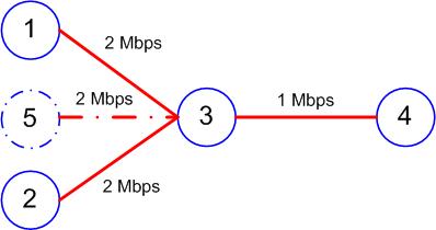
Figure 2
To extract the files type: tar xvf task2.tar
In the first part of Task2 simulations, we'll use 3 blackbox TCP implementations: TCP_A, TCP_B, and TCP_C. In Tcl scripts, their sender agents are created by using Agent/TCP/tcp_A, Agent/TCP/tcp_B, Agent/TCP/tcp_C, respectively. Their corresponding receive agents have to be Agent/TCPSink/Sink_A, Agent/TCPSink/Sink_B, and Agent/TCPSink/Sink_C. We know these 3 TCP variants implement TCP Tahoe, TCP Reno, and TCP SACK. But it is unknown which implements the one we want. NS2 simulator doesn't know what these agents are, but our own simulator BNS knows. Basically, BNS can handle all Tcl scripts for NS2 simulations, as well as those scripts that use the four TCP blackboxes. You can download the BNS executable file from the web site of Project 2 (http://inst.eecs.berkeley.edu/~ee122/project/proj2_index.html).
Together with the simulator NSB, we also provide three sample Tcl files that simulate the given network: tcp_A.tcl, tcp_B.tcl, tcp_C.tcl. They use TCP_A, TCP_B, and TCP_C, respectively. The Tcl simulation script "tcp_x.tcl", where "x" is one of "A", "B", and "C", produces following output trace files:
· tcp_x.nam and tcp_x.tr: their formats are defined by NS2. (refer http://www.isi.edu/nsnam/ns/doc/node272.html, and http://www.isi.edu/nsnam/ns/doc/node565.html)
· tcp_x_throughput.tr: each entry looks like "[time] [TCP throughput in link from node 3 to node 4]".
· tcp_x_drop.tr: each entry looks like "[time] [number of dropped packets in the buffer of link from node 3 to node 4]".
· tcp_x_cwind.tr: each entry looks like "[time] [congestion window (packets) of TCP sender]".
· tcp_x_seq.tr: each entry looks like "[time] [max (packet) seq number sent by TCP sender]".
· tcp_x_ack.tr: each entry looks like "[time] [highest ACK received by TCP sender]".
Plotting related figures (congestion window (packets) of TCP sender as a function of time, max (packet) sequence number sent by TCP sender as a function of time, highest ACK received by TCP sender as a function of time, and number of dropped packets in the buffer of link from node 3 to node 4 as a function of time) from these trace files will help you guess the TCP variant that each of these blackboxes implements. Usually the traffic scenario we provide in the sample Tcl scripts will generate enough information for you to recognize the TCP variant. However, if you want to get more information, you may modify the sample Tcl scripts to change the traffic so that expected TCP behavior will be triggered.
A good reference for this project is Fall and Floyd's paper, "Simulation-based Comparisons of Tahoe, Reno, and SACK TCP" ( ps, pdf).
(a) Run all these Tcl simulation scripts. Based on the observation on the behavior of these TCP blackboxes, identify the blackbox for each of those three TCP variants.
(b) For each blackbox implementation save the following graphs: highest ACK received by TCP as a function of time, cwnd as a function of time.
(c) For the blackbox corresponding to TCP Tahoe: At what time is additive increase invoked for the second time? What is the approximate beginning time that multiplicative decrease is invoked for the third time? What is the approximate beginning time that fast retransmit is invoked for the first time?
(d) For the blackbox for TCP Reno: What is the approximate beginning time that fast recovery is invoked for the first time? What is the approximate time interval that additive increase is invoked for the second time?
(e) Which of the TCP variants achieves the highest throughput and why?
Another
variant of TCP, FAST TCP: implements an alternative
congestion control scheme:
·
First, it is an
equation-based algorithm and hence eliminates packet-level oscillations
·
Second, it uses
queueing delay as the primary measure of congestion, which can be more reliably
measured by end hosts than loss probability in fast long-distance networks.
·
Third, it has a
stable dynamics and achieves weighted proportional fairness in equilibrium.
Fast TCP was designed to achieve higher throughput in high-bandwidth and delay networks
The simulation scenario provided in Reno_Fast_tcp1.tcl and Reno_Fast_tcp2.tcl sets up the same network topology used above, but with different traffic: there is one one TCP/Reno source and one TCP/Fast source. The network topologies created in the two scripts are the same – the only difference is the bandwidth and delay of the links
(f) (task2.pdf) Run the two scripts. What is the throughput for TCP/Fast and TCP/Reno in each case. When does TCP/Fast outperform TCP/Reno (script 1 or 2). Why?
Queueing SchemesIn Drop tail, a router serves incoming packets in the arrival order, and when the buffer is full, the newly arriving packet is simply discarded.
Task 2 uses a similar network topology in Figure 1 (Task 1), but instead of only 2 nodes, there are 10 nodes and 10 TCP traffic flows. Now the TCP/FTP flow from node 1 through 10 starts at 0.1 seconds. There is no background traffic.
RED is designed to cooperate with the congestion control mechanism of TCP. It detects the beginning of congestion by monitoring the average buffer occupancy at the router, and notifies the connections by intentionally dropping packets at a certain probability. RED sets the packet dropping probability by a function of buffer occupancy (average queue size).
So far we have used Drop-tail congestion notification schemes In the next section we will provide you will scripts that implement drop tail, RED
(g) Run the simulations and identify which one is drop tail, and which one is RED. Give supporting evidence for your choice
5 Checkpoint, Submission and Grading
5.1 Checkpoint
This project is handed out on October 19, and is due on November 2
(11.59PM). You have two weeks to work on it. You are strongly
urged to start your project as early as possible! Be aware that you don't
have any slip day for homeworks and projects.
5.2 Submission
The project can only be submitted online. To submit your files, create
a directory, first copy the relevant files into that directory. Then go
into that directory and type
- % submit proj2
- task1.pdf, task1_b.tcl, task1_c.tcl, task1_d.tcl
- task2.pdf
- Task 1 (total 10 pts)
- Part (a) (total 0.5 pt)
- What is the packet loss rate of the two TCP flows? What is the ratio of throughput between the two packets?
- Part (b) (total 2 pts)
- task1_b.tcl (1 pt)
- Give the packet loss rate of the two TCP/FTP flows (0.5 pt)
- Which flow uses more bandwidth in the bottleneck link from node 3 to node 4? (0.5 pt)
- Part (c) (total 3.5 pts)
- task1_c.tcl (1 pt)
- Give the total bytes of traffic for each flow. (0.5 pt)
- How does the packet loss rate change? (0.5 pt)
- Do both flows receive a "fair share" of the available bandwidth of the bottleneck link? (0.5 pt)
- What is the reason? (1 pt)
- Part (d) (total 4 pts)
- task1_d.tcl (1 pt)
- Give the total bytes of TCP for each flow (1 pt)
- task1_d_total.awk (Awk script to compute the total bytes of traffic for part d) (1 pt)
- Do all TCP/FTP flows receive a "fair share" of the available bandwidth of the bottleneck link? Why or why not? (1 pt)
- Task 2 (total 30 pts)
- Part (a) (total 6 pts)
- Which one is TCP Tahoe (2 pt)
- Which one is TCP Reno (2 pt)
- Which one is TCP SACK (2 pt)
- Part (b) (total 3 pts)
- All plots (1 pt)
- Part (c) (total 6 pts)
- (2 pts each question) For the blackbox corresponding to TCP Tahoe: At what time is additive increase invoked for the second time? What is the approximate beginning time that multiplicative decrease is invoked for the third time? What is the approximate beginning time that fast retransmit is invoked for the first time?
- Part (d) (total 4 pts)
- 2pts For the blackbox for TCP Reno: What is the approximate beginning time that fast recovery is invoked for the first time?
- 2pts What is the approximate time interval that additive increase is invoked for the second time?
- Part (e) (total 3 pts) answer + reason
- Part (f) (total 4 pts) answer + reason
- Part (g) (total 4 pts) answer + reason
Last updated: 10/26/2004