Extended Ray Tracer

Assignment Results:

For our final project we decided to extend our ray tracer from HW5 by adding more features and optimizing render time. Before starting, our ray tracer was already using an octree acceleration structure and we had already implemented soft shadows, anti aliasing, refraction, reading in obj files, and applying textures to triangles. For more details on what he had already implemented, click here. In order to use some of these features, you would need to add certain commands in the scene files. These new commands will be explained in the following sections but you can see a list of them and their brief explanations below.

Smooth Shading

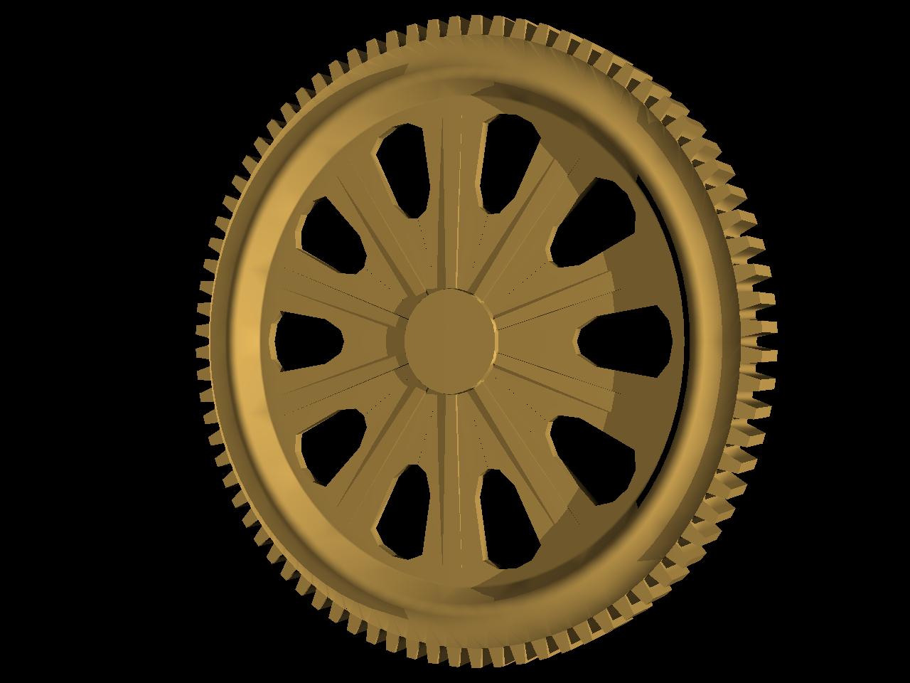
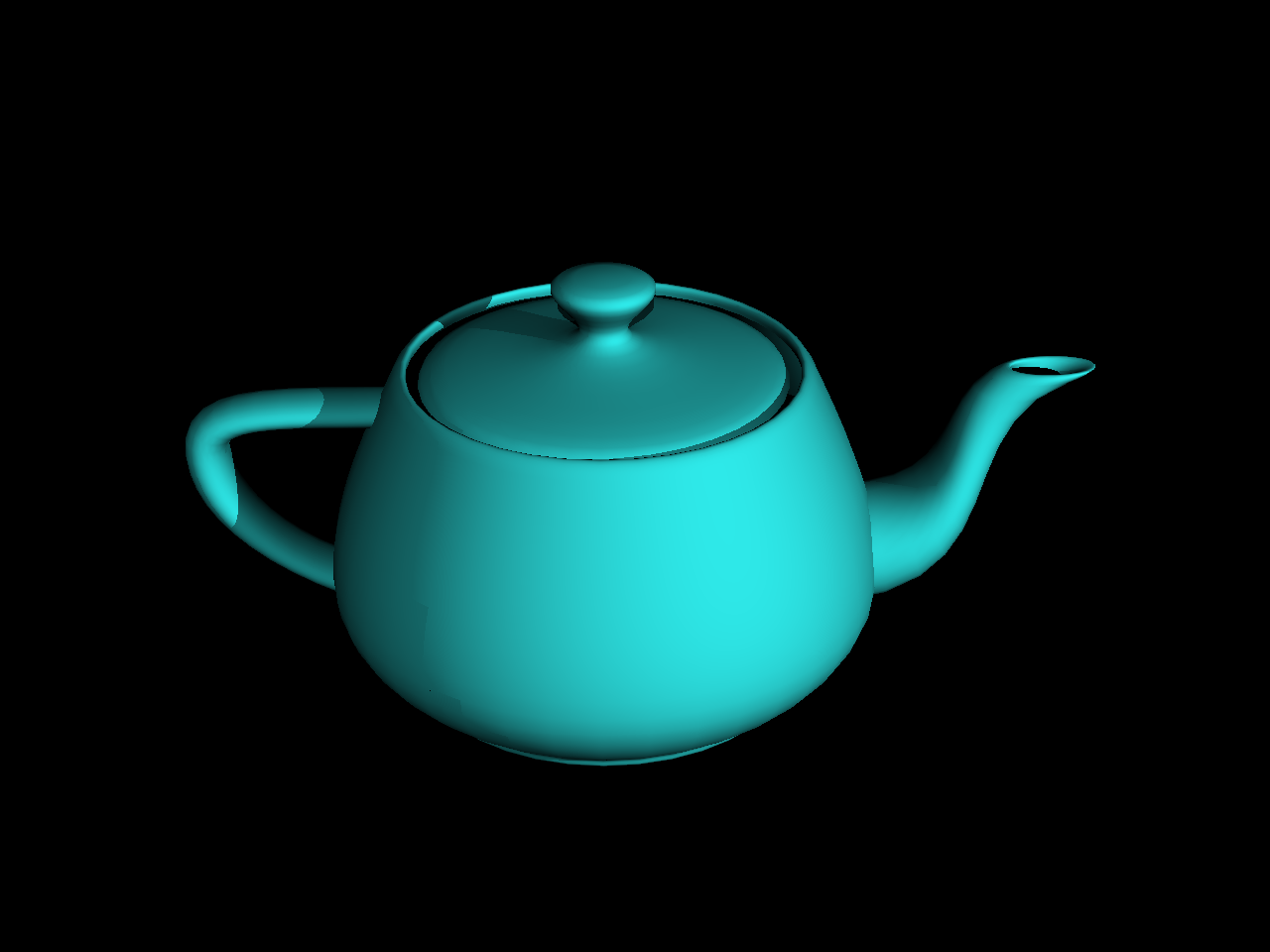
We implemented smoothing of normals for object files that we import. In order to do this, the normals of all the faces a vertex is part of are calculated and then combined to create a single vertex normal. An additional consideration is the preservation of sharp edges on the object. To that end, when specifying a smooth object, one also specifies a threshold angle used when calculating vertex normals. If the angles of two faces differ by more than the threshold, a separate vertex is created for each of the faces. This allows objects to be smoothed without ruining the intentionally sharp edges.

Added Command:

Usage	Explanation
objSmooth <objName> <thresholdAngle>	Imports the .obj file specified by objName and smooths it, preserving edges with angle greater than the specified threshold

Unsmoothed	Smoothed

Improved Acceleration Structure

We improved upon our octree acceleration structure from Homework 5 in two main ways. First, we tuned some of it's parameters across a variety of scenes to see which provided fastest render times. Specifically, we changed the threshold of objects in a bounding box below which the octree would stop recursing and be a leaf. We also changed the maximum depth of the octree. Together these parameters tweaked with the trade off between more ray axis-aligned-bounding-box (AABB) intersections versus more object (triangle and sphere) intersections. We found cutting off recursion when there were 3 or fewer objects in the bounding box and limiting the maximum recursion to 6 layers to be the generally optimal parameters. In addition, we optimized our ray-AABB intersection test, as it is one of the most called methods in our code. We used Plücker coordinates for a fast implementation of determining whether or not a ray intersected an AABB and then found the distances to each of the 3 closer planes of the box in the traditional method. While not nearly as impactful as our optimizations from profiling observations, these changes did decrease the render time.

Optimizations

We profiled our code to find bottlenecks and optimize the routines that we were spending the most time in. By compiling with the '-pg' flag and using gprof, we identified the transformations taking place in a lot of the triangle methods as taking a long time. In order to speed this up, we pre-transformed the triangle, storing the transformed vertices and then never using the transformation matrix again. This is much faster than the previous method of storing the untransformed vertex coordinates and transforming rays and normals back and forth. We also turned on compiler optimizations with the '-O3' flag, which again led to a significant speed up in render time. Below is the comparison between render times with our un-optimized ray tracer from homework 5 and our optimized ray tracer.

Scene File	HW5 Ray Tracer	Optimized Ray Tracer
scene5.test (One thousand spheres)	10.066 Seconds	1.778 Seconds
scene6.test (Cornell box with three spheres and two cubes)	16.831 Seconds	2.184 Seconds
scene7.test (Stanford dragon)	24.785 Seconds	1.910 Seconds

Normal Mapping

Our ray tracer can use a texture as a normal map, simulating bumps and tessellation on a smooth surface. Having added support for textures in Homework 5, implementing the use of normal maps became a matter of creating the matrix that would transform all incoming and outgoing vectors into tangent space. As we only support textures on triangles, normal maps are similarly only available on triangles. Since the effect of normal maps rely on how light interacts with the surface, it's easiest to see when the light or surface is moving. To that end, we created this animation in which a point light moves in front a flat normal mapped surface. Note how the surface appears spherical.

Added Commands:

Usage	Explanation
normalMap <normalMapName>	loads in the texture specified by normalMapName and uses it as the normal map for all future triangles until the normalMap or clearNormalMap command is encountered
clearNormalMap	All future triangles have no normal map until the normalMap command is encountered

Depth of Field

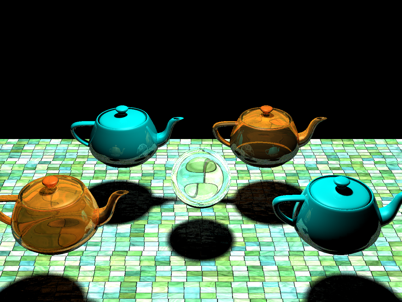
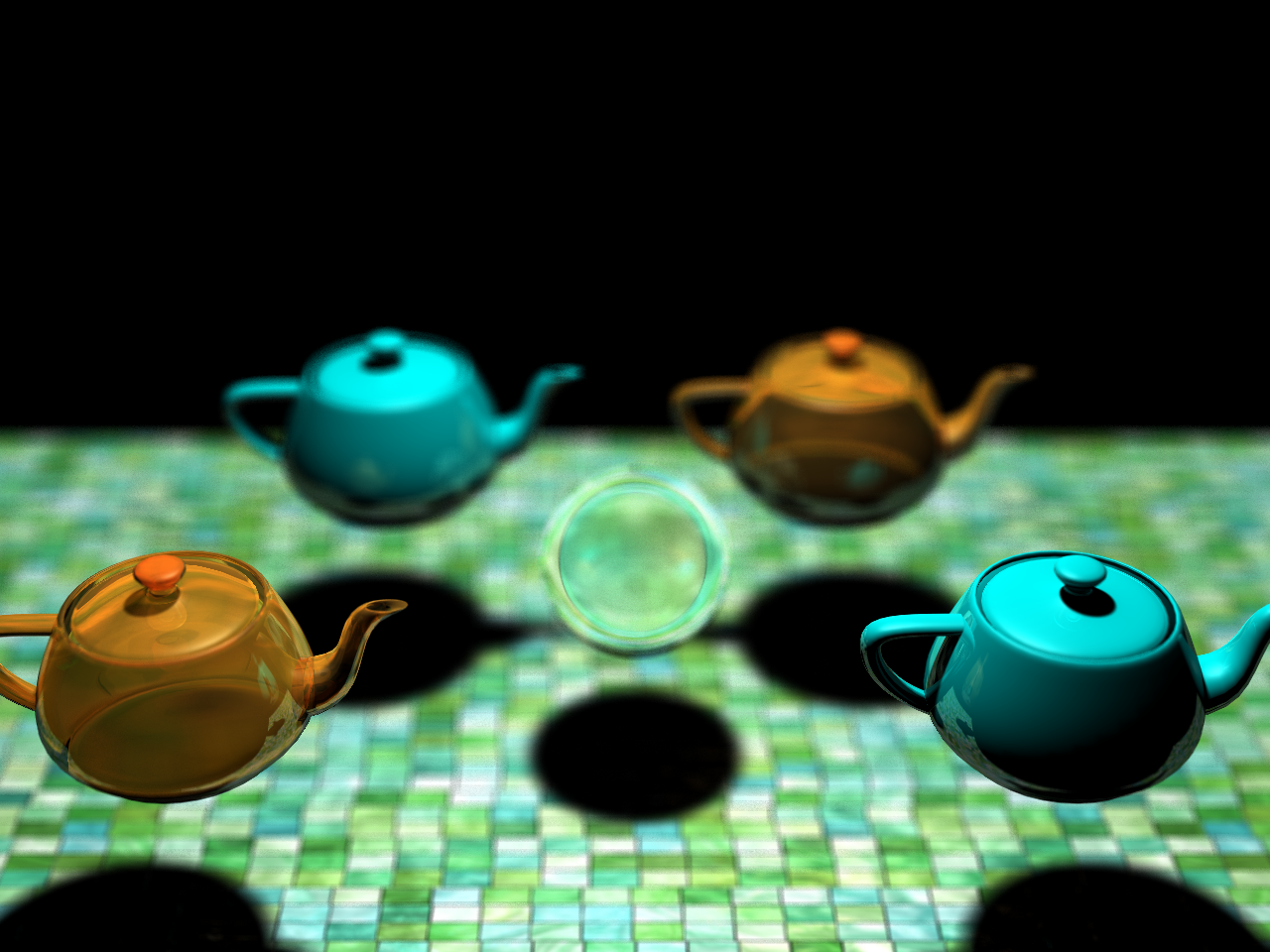
Depth of field is used to simulate the inaccuracies and limitations of a real optical system, thereby creating more realistic images. In an actual optical system such as a camera or your eye, a lens focuses incoming rays onto a single point or screen, such as film or your retina. However, the lens is only able to focus rays originating from a single distance, and rays from objects that are nearer or farther than that distance don't get focused to a single point but rather spread out across the screen, resulting in blur. This effect is known as depth of field. We simulate depth of field by calculating the point in space at which a focused ray would hit, then shoot many rays with perturbed origins through that point. The final value of the pixel is the average of these rays. Thus, if there is an object at or near the focal point, all of the rays will hit about the same place and the object will look in focus. If there is nothing at the focal point or something between the pixel and the focal point, the rays will hit very different areas of the scene and the image will appear blurry. In our implementation, an aperture corresponds to the radius of the lens we are simulating. Concretely aperture is the range over which ray origins are moved; in practice it controls how blurry an image gets (higher aperture means more blur). Focal length is the distance from the camera at which an object will be perfectly in focus. Number of rays controls how many rays are sent out for each pixel, which corresponds to the quality of the blur: fewer rays renders faster but results in noisy speckled blur.

Added Commands:

Usage	Explanation
DOF <aperture size> <focal length> <num Rays>	The aperture controls the strength of the blurring effect, focalLength controls the distance at which objects are in focus, and numRays determines how many rays are used per pixel

These images demonstrate the depth of field effect. Click an image to view a larger version.

No depth of field	Near focus depth of field	Far focus depth of field

This video demonstrates depth of field by changing the focal length from near to far.

Distributed Rendering

In order to render large or complicated images, such as those that use depth of field or anti-aliasing, at a reasonable speed, we wrote a script that rendered small chunks of the image on the hive machines and then transferred them back to our machine. By utilising the combined power of most or all of the hive machines, we achieved dramatic speed ups, opening the door to rendering much more complicated scenes and animations in the give time frame. The depth of field animation above, which is 96 frames long, took about 4 minutes to render each frame when distributed across the hive cluster. On a 4 core hyper-threaded machine such as we have, a single frame would have taken about 3 hours; at that speed, the entire animation would have taken 12 days. This distributed rendering allowed us to render the entire animation in 6 hours. In order to not monopolize all of the resources of the 330 Soda lab, before each frame, we checked the computers' load averages to make sure that no one else was using the machines in any significant way, so that we wouldn't be making the computer unusable or too slow. This also helped our render times, as if a machine was splitting processing power with other users, that single patch of the image would render slower and would hold up the rest of the process.

Animation

In order to produce animations, we wrote a script that would take in an animation file, create a series of scene files (one for each frame of the animation), render all of the scenes, and then combine the final product into a movie file. The animation file was almost exactly the same as the scene files it generated, except it allowed for parameters to be changed over time. Our animation file format allowed key frames to be set for commands, creating an expressive and flexible system for specifying change over time. For instance, to make an object move in a square, one could use the following lines to add an animated translate before the object definition:

animate translate
0:0 0 0
24:0 1 0
48:1 1 0
72:1 0 0
96:0 0 0
endAnimate

The animation script automatically does linear interpolation between the values to create the intermediate frames. This means that only commands with numerical parameters can be animated currently. Finally, we used the linux program avconv to stitch the images together at 24 frames per second to create the final video. Examples of animations generated by this procedure can be seen in the YouTube videos embedded on this page.

Added Commands:

Usage	Explanation
animationFrames <startFrame> <endFrame>	Specifies the range of frames over which the animation should be rendered
animate <command>	Specifies a command to be animated and signals the beginning of a list of key frames
<frame>:<parameters>	A key frame that specifies what the parameters should be for the command being animated at the given frame number
endAnimate	Signifies the end of a list of key frames

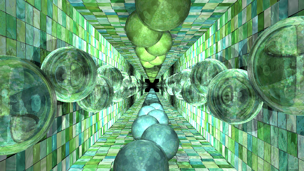
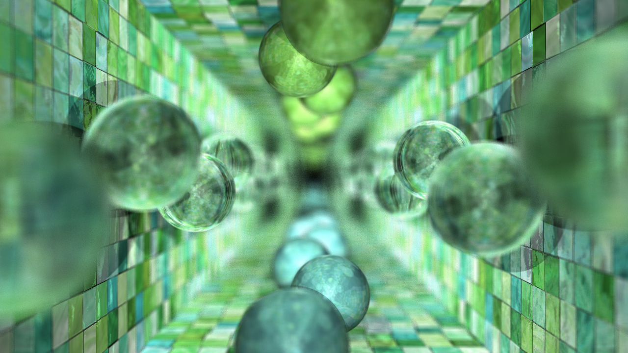
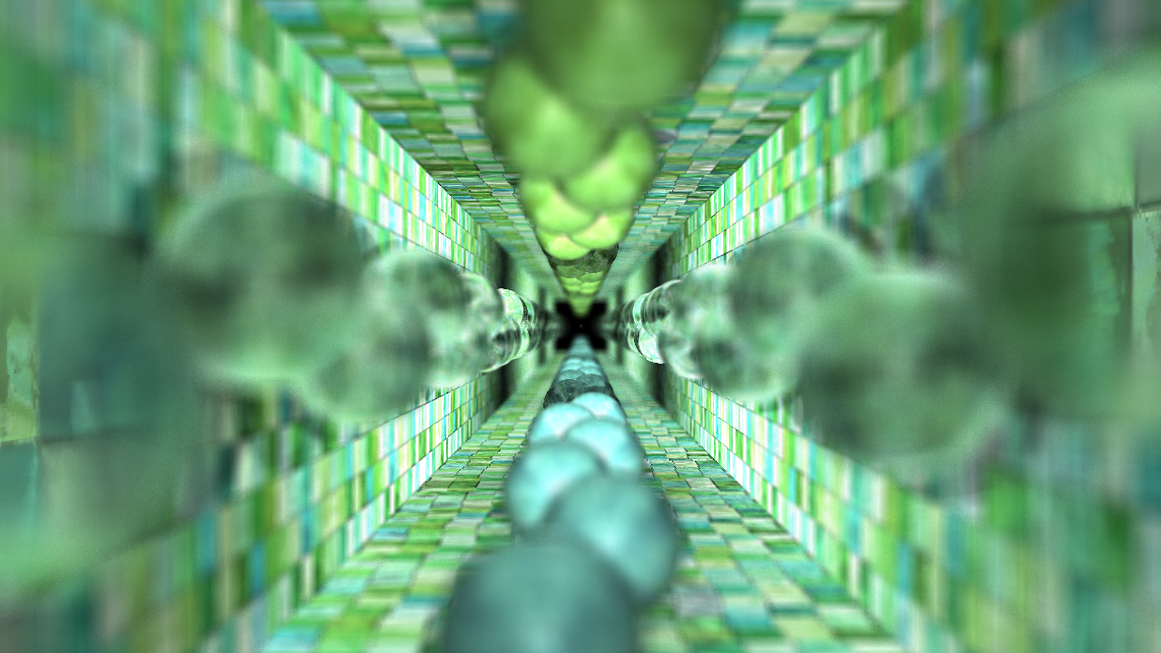
Put it all Together

We combined everything into one animation. We have layers of spheres in a hallway that rotate about the origin in alternating directions. The scene has a depth of field and the hallway is textured and bump mapped. The camera is also animated to move through the center of rotation. We rendered each frame to be 1280px720p and converted the image sequence into an avi at 24fps. The original video (which can be downloaded here) has better quality than the youtube video below so we recommend seeing the embedded video in 720p.

API

This is a comprehensive list of all of the commands we have added to the scene file format defined in the project specifications

Arguments are specified in angled brackets

Usage	Explanation
animationFrames <startFrame> <endFrame>	Specifies the range of frames over which the animation should be rendered
animate <command>	Specifies a command to be animated and signals the beginning of a list of key frames
<frame>:<parameters>	A key frame that specifies what the parameters should be for the command being animated at the given frame number
endAnimate	Signifies the end of a list of key frames
DOF <aperture size> <focal length> <num Rays>	The aperture controls the strength of the blurring effect, focalLength controls the distance at which objects are in focus, and numRays determines how many rays are used per pixel
texture <filename>	loads in the texture specified by filename and uses it as the texture for all future triangles until the texture or clearTexture is encountered
clearTexture	All future triangles have no texture until the texture command is encountered
normalMap <normalMapName>	loads in the texture specified by normalMapName and uses it as the normal map for all future triangles until the normalMap or clearNormalMap command is encountered
clearNormalMap	All future triangles have no normal map until the normalMap command is encountered
objSmooth <objName> <thresholdAngle>	reads in the object file specified by objName and renders it with the specified threshold angle
area <x> <y> <z> <rad> <r> <g> <b>	define an area light producing soft shadows with center at (x,y,z) with radius rad emitting a light with color (r,g,b)
directionalSoft <x> <y> <z> <r> <g> <b>	makes a directional light with direction (x,y,z) to the light source with the color (r,g,b) producing soft shadows
antiAlias <x>	subdivides each pixel into x*x grid and finds the color of a random point in each section and averages the values found to get the final color of the pixel
tint <r> <g> <b>	changes the color of refractions
refract <eta>	makes the following objects have the eta of refraction