Final Project: Extended Ray Tracer

Partners

Justin Uang            cs184-ax     http://inst.cs.berkeley.edu/~CS184-ax/hw6/hw6.html
Christine Nguyen       cs184-aw     http://inst.cs.berkeley.edu/~CS184-aw/

Summary

For our final project, we extended our ray tracer to be able to generate images with refractions, soft shadows, depth of field , and motion blur. We also spent a lot of time improving the KD-Tree implemention to use the surface area heuristic for splitting.

Original Ray Tracer

Our original ray tracer had the following capabilities:

Original Features

Camera: Users could specify camera location by entering the command
```
camera lookfromx lookfromy lookfromz lookatx lookaty lookatz upx upy upz fov
```
in a .test scene file.
Parser: Users could supply a file at command line describing a scene and our ray tracer was able to parse the file and generate a scene. Typing:
```
./ray_tracer input.test
```
at command line would run the ray tracer on the input file.
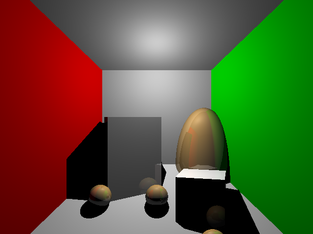
Reflections: Our original ray tracer could handle recursive ray tracing to an arbitrary depth (the default was 3) which let us generate images with reflections.
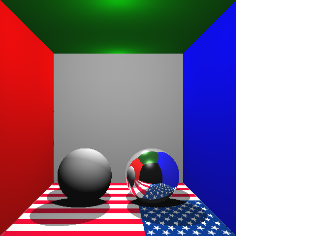
Texture Mapping: Textures could be mapped to squares in our original ray tracer.
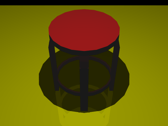
OBJ Parser: OBJ files could be read in and images of objects specified by OBJ files could be rendered
Jittering: Jittering was implemented in the original version of our ray tracer
Unfinished KD-tree: An imperfect kd-tree was implemented in the original version of our ray tracer.

KD-Tree

Our implementation of the KD-Tree in hw5 had a few critical bugs. For this part of the project, we fixed the initial implementation of the KD-Tree and implemented the Surface Area Heuristic

Bugs

When testing a ray against a node in the kd-tree, we verify that the intersection of the ray and the objects that lie in the box is inside the box. Before, if the intersection occurred outside of the box, we would consider it a hit before traversing other boxes which may have objects that lie closer.
When the origin of the ray is exactly at 0, and there is a node in the KD-Tree whose bounding box had an edge on 0, the ray would not be intersect the box. We fixed this by adding an epsilon to each ray before the intersection tests.

Surface Area Heuristic

In addition, instead of splitting on the median of a bounding box, we implemented a smarter rule using the Surface Area Heuristic

The original algorithm looked like this (it simply cycled on the axis parameter):

split = (voxel.max[axis] + voxel.min[axis]) / 2;

Now, we follow the Surface Area Heuristic which calculates the cost of a split:

cost = Ctraversal + area * prims * Cintersect

Thus, we loop over all the possible split points (defined by the boundaries of the triangles and spheres), and calculate the split point that minimizes the cost. This also gives us a clean way to stop building the KD-Tree. Before, we set a threshold such that the KD-Tree could just grow beyond a certain depth. Now, we stop when:

cost (no split) < cost (left split) + cost (right split)

The following image was the one provided by the class (scene5.bmp) that has many polygons. Because of the speedups in our kdtree implementation, we were able to run it with jittering and have it finish in a reasonable amount of time (9 ray jittering):

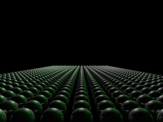
Results (9 ray jittering, OpenMP on a 12 core machine):

Number of intersection tests using naive median split method: 148,071,898 (6.76 seconds)

Number of intersection tests using surface area heuristic: 7,792,562 (52.53 seconds)

Although the overhead of constructing the KD-Tree is greater when using the Surface Area Heuristic, it partitions space to have more empty blocks, greatly reducing the number of ray-intersection tests.

We also tested on scene7.bmp, also given by the class.

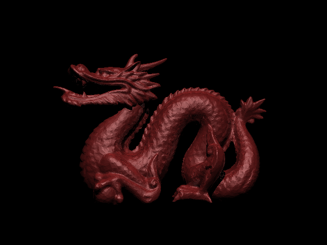
Results (OpenMP on a 12 core machine):

Number of intersection tests using naive median split method: 134,867,354 (8.09 seconds)

Number of intersection tests using surface area heuristic: 12,165,520 (18.97 seconds)

Using the surface area heuristic results in less than 1/10 of the intersection tests, it takes longer because of the overhead of creating the KD-Tree.

Refractions

We implemented recursive ray tracings with refractions using Snell's law and the basic refractions equations described in the paper by Bram de Greve. According to the paper, the basic refraction ray can be given by:

n = n1/n2
sin(theta)^2 = n^2 (1-cos^2(theta))
refracted_ray = n*I + (n*cos(theta) - sqrt(1 - sin^2(theta))) * N

where N is the normal, I is the incident ray, and theta is the incident angle. n1 and n2 are the indices of refractions for the materials that the light ray is exiting and entering respectively. To indicate that an object should refract light, before declaring the object in the test file, specify the material properties:

transparency 1
refraction_index 1.5

The number following the "transparency" command should be greater than 0 if the object is transparent, and the number following the "refraction index" command should specify the index of refraction for the object.

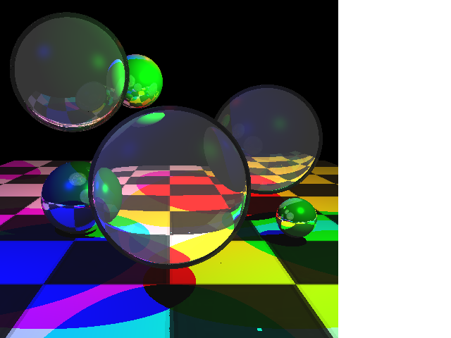
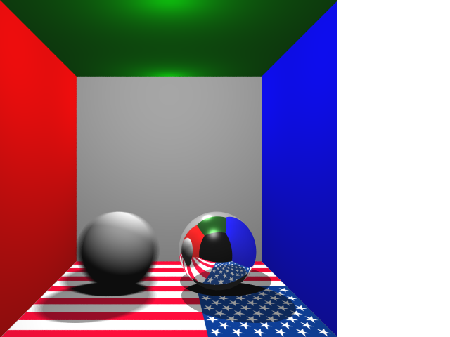
Here are some examples of images with refractive sphere that we generated:

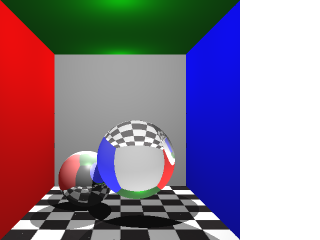$Refraction-cornell$ An image of a refractive sphere in a cornell box

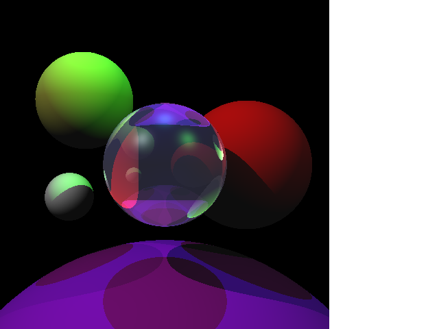$Refraction2.1$ An image of a refractive sphere among several spheres

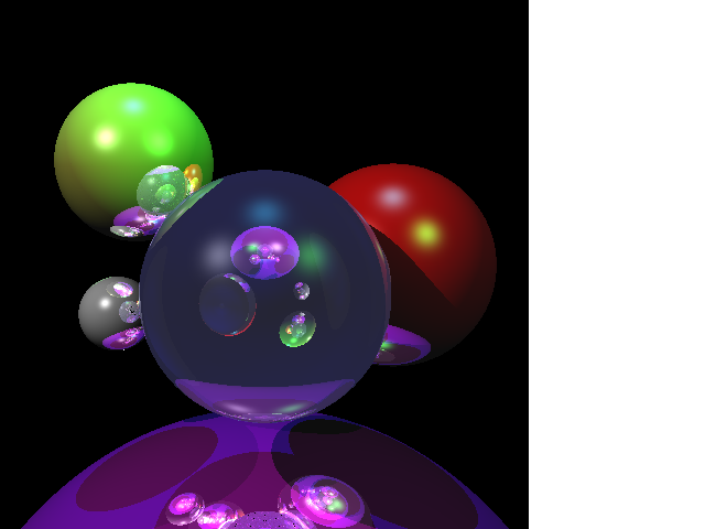$Refraction2$ The same image with reflections enabled

As a small feature, we extended our ray tracer to be able to generate images of "bubbles" or hollow spheres. Bubbles

Soft Shadows

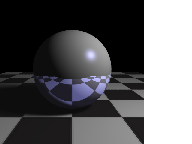
We implemented soft shadows using a jittering method. At an intersection on the surface, we shoot rays to the light source, but assume that the light source is an area source. We put a grid around the light source, and shoot into random locations within each cell in the grid.

To turn it on, use the following commands in the input file:

shadows 1    # Turns on hard shadows
shadows 2    # Turns on soft shadows

Here is a sample image (9 ray jittering, 9 ray soft shadows):

Depth of Field

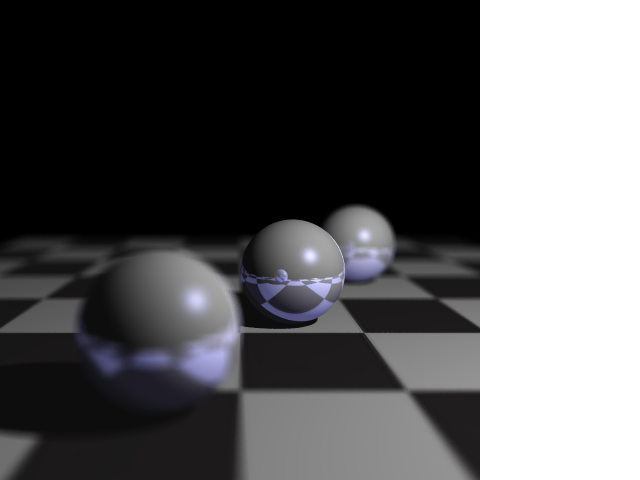
Depth of Field was implemented by placing a jittering grid around the camera origin, and then sampling points within each cell of the jittering grid. Each one of these points is the origin of a ray whose direction directs it to the point on the focal plane that the original, unperturbed point would hit.

More precisely,

focal_point = primary_ray.origin + focal_length * primary.direction
for (jittered_location in jitter_grid)
{
  Ray jittered_ray;
  jittered_ray.origin = jittered_location;
  jittered_ray.direction = normalize(focal_point - jittered_ray.origin)
}

To activate depth of field, use the following commands:

camera_aperture 1
camera_focal_length 50

dof 5    # Sets the dimension of the jitter grid (uses 5 * 5 samples)

Here is a sample image (9 ray jittering, 25 depth of field rays):

Motion Blur

We implemented motion blur by sampling over time. Each object was expanded to have the a velocity attribute. The camera was also given a shutter_speed attribute. motion_blur_samples defines many samples are taken (in time space) to simulate the motion blur effect:

camera_shutter_speed 0.5
motion_blur_samples 5

...

vel 1 0 0
sphere ...

The pseudocode for the effect goes like this:

for (time_sample in time_samples)
{
  for (node in all_nodes)
  {
    node.translate (time_sample * node.velocity)
  }

  render_image()
}

average_rendered_images()

Here is a sample image (9 ray jittering, 5 time samples): Motion Blur