>>> r = range(10000, 1000000000)
>>> r[45006230]
45016230

4.2.1   Python Iterators

The Python iterator interface includes two messages. The __next__ message queries the iterator for the next element of the underlying series that it represents. In response to invoking __next__ as a method, an iterator can perform arbitrary computation in order to either retrieve or compute the next element in an underlying series. Calls to __next__ make a mutating change to the iterator: they advance the position of the iterator. Hence, multiple calls to __next__ will return sequential elements of an underlying series. Python signals that the end of an underlying series has been reached by raising a StopIteration exception during a call to __next__.

The Letters class below iterates over an underlying series of letters from a to d. The member variable current stores the current letter in the series, and the __next__ method returns this letter and uses it to compute a new value for current.

>>> class Letters(object):
        def __init__(self):
            self.current = 'a'
        def __next__(self):
            if self.current > 'd':
                raise StopIteration
            result = self.current
            self.current = chr(ord(result)+1)
            return result
        def __iter__(self):
            return self

The __iter__ message is the second required message of the Python iterator interface. It simply returns the iterator; it is useful for providing a common interface to iterators and sequences, as described in the next section.

Using this class, we can access letters in sequence.

>>> letters = Letters()
>>> letters.__next__()
'a'
>>> letters.__next__()
'b'
>>> letters.__next__()
'c'
>>> letters.__next__()
'd'
>>> letters.__next__()
Traceback (most recent call last):
  File "<stdin>", line 1, in <module>
  File "<stdin>", line 12, in next
StopIteration

A Letters instance can only be iterated through once. After its __next__() method raises a StopIteration exception, it continues to do so from then on. There is no way to reset it; one must create a new instance.

Iterators also allow us to represent infinite series by implementing a __next__ method that never raises a StopIteration exception. For example, the Positives class below iterates over the infinite series of positive integers. The built-in next function in Python invokes the __next__ method on its argument.

>>> class Positives(object):
        def __init__(self):
            self.current = 1;
        def __next__(self):
            result = self.current
            self.current += 1
            return result
        def __iter__(self):
            return self
>>> p = Positives()
>>> next(p)
1
>>> next(p)
2
>>> next(p)
3

4.2.2   For Statements

The for statement in Python is designed to operate on iterators. Objects are iterable (an interface) if they have an __iter__ method that returns an iterator. Iterable objects can be the value of the <expression> in the header of a for statement:

for <name> in <expression>:
    <suite>

To execute a for statement, Python evaluates the header <expression>, which must yield an iterable value. Then, the __iter__ method is invoked on that value. Until a StopIteration exception is raised, Python repeatedly invokes the __next__ method on that iterator and binds the result to the <name> in the for statement. Then, it executes the <suite>.

>>> counts = [1, 2, 3]
>>> for item in counts:
        print(item)
1
2
3

In the above example, the counts list returns an iterator from its __iter__() method. The for statement then calls that iterator's __next__() method repeatedly, and assigns the returned value to item each time. This process continues until the iterator raises a StopIteration exception, at which point execution of the for statement concludes.

With our knowledge of iterators, we can implement the execution rule of a for statement in terms of while, assignment, and try statements.

>>> items = counts.__iter__()
>>> try:
        while True:
            item = items.__next__()
            print(item)
    except StopIteration:
        pass
1
2
3

Above, the iterator returned by invoking the __iter__ method of counts is bound to a name items so that it can be queried for each element in turn. The handling clause for the StopIteration exception does nothing, but handling the exception provides a control mechanism for exiting the while loop.

4.2.3   Generators and Yield Statements

The Letters and Positives objects above require us to introduce a new field self.current into our object to keep track of progress through the sequence. With simple sequences like those shown above, this can be done easily. With complex sequences, however, it can be quite difficult for the __next__ method to save its place in the calculation. Generators allow us to define more complicated iterations by leveraging the features of the Python interpreter.

A generator is an iterator returned by a special class of function called a generator function. Generator functions are distinguished from regular functions in that rather than containing return statements in their body, they use yield statement to return elements of a series.

Generators do not use attributes of an object to track their progress through a series. Instead, they control the execution of the generator function, which runs until the next yield statement is executed each time the generator's __next__ method is invoked. The Letters iterator can be implemented much more compactly using a generator function.

>>> def letters_generator():
        current = 'a'
        while current <= 'd':
            yield current
            current = chr(ord(current)+1)

>>> for letter in letters_generator():
        print(letter)
a
b
c
d

Even though we never explicitly defined __iter__ or __next__ methods, the yield statement indicates that we are defining a generator function. When called, a generator function doesn't return a particular yielded value, but instead a generator (which is a type of iterator) that itself can return the yielded values. A generator object has __iter__ and __next__ methods, and each call to __next__ continues execution of the generator function from wherever it left off previously until another yield statement is executed.

The first time __next__ is called, the program executes statements from the body of the letters_generator function until it encounters the yield statement. Then, it pauses and returns the value of current. yield statements do not destroy the newly created environment, they preserve it for later. When __next__ is called again, execution resumes where it left off. The values of current and of any other bound names in the scope of letters_generator are preserved across subsequent calls to __next__.

We can walk through the generator by manually calling ____next__():

>>> letters = letters_generator()
>>> type(letters)
<class 'generator'>
>>> letters.__next__()
'a'
>>> letters.__next__()
'b'
>>> letters.__next__()
'c'
>>> letters.__next__()
'd'
>>> letters.__next__()
Traceback (most recent call last):
  File "<stdin>", line 1, in <module>
StopIteration

The generator does not start executing any of the body statements of its generator function until the first time __next__ is invoked. The generator raises a StopIteration exception whenever its generator function returns.

4.2.4   Iterables

In Python, iterators only make a single pass over the elements of an underlying series. After that pass, the iterator will continue to raise a StopIteration exception when __next__ is invoked. Many applications require iteration over elements multiple times. For example, we have to iterate over a list many times in order to enumerate all pairs of elements.

>>> def all_pairs(s):
        for item1 in s:
            for item2 in s:
                yield (item1, item2)

>>> list(all_pairs([1, 2, 3]))
[(1, 1), (1, 2), (1, 3), (2, 1), (2, 2), (2, 3), (3, 1), (3, 2), (3, 3)]

Sequences are not themselves iterators, but instead iterable objects. The iterable interface in Python consists of a single message, __iter__, that returns an iterator. The built-in sequence types in Python return new instances of iterators when their __iter__ methods are invoked. If an iterable object returns a fresh instance of an iterator each time __iter__ is called, then it can be iterated over multiple times.

New iterable classes can be defined by implementing the iterable interface. For example, the iterable LetterIterable class below returns a new iterator over letters each time __iter__ is invoked.

>>> class LetterIterable(object):
        def __iter__(self):
            current = 'a'
            while current <= 'd':
                yield current
                current = chr(ord(current)+1)

The __iter__ method is a generator function; it returns a generator object that yields the letters 'a' through 'd'.

A Letters iterator object gets "used up" after a single iteration, whereas the LetterIterable object can be iterated over multiple times. As a result, a LetterIterable instance can serve as an argument to all_pairs.

>>> letters = LetterIterable()
>>> all_pairs(letters).__next__()
('a', 'a')
>>> all_pairs(letters).__next__()
('a', 'a')

4.2.5   Streams

Streams offer another way to represent sequential data implicitly. A stream is a lazily computed recursive list. Like the Rlist class from Chapter 3, a Stream instance responds to requests for its first element and the rest of the stream. Like an Rlist, the rest of a Stream is itself a Stream. Unlike an Rlist, the rest of a stream is only computed when it is looked up, rather than being stored in advance. That is, the rest of a stream is computed lazily.

To achieve this lazy evaluation, a stream stores a function that computes the rest of the stream. Whenever this function is called, its returned value is cached as part of the stream in an attribute called _rest, named with an underscore to indicate that it should not be accessed directly. The accessible attribute rest is a property method that returns the rest of the stream, computing it if necessary. With this design, a stream stores how to compute the rest of the stream, rather than always storing it explicitly.

>>> class Stream(object):
        """A lazily computed recursive list."""
        class empty(object):
            def __repr__(self):
                return 'Stream.empty'
        empty = empty()
        def __init__(self, first, compute_rest=lambda: empty):
            assert callable(compute_rest), 'compute_rest must be callable.'
            self.first = first
            self._compute_rest = compute_rest
            self._rest = None
        @property
        def rest(self):
            """Return the rest of the stream, computing it if necessary."""
            if self._compute_rest is not None:
                self._rest = self._compute_rest()
                self._compute_rest = None
            return self._rest
        def __repr__(self):
            return 'Stream({0}, <...>)'.format(repr(self.first))

A recursive list is defined using a nested expression. For example, we can create an Rlist that represents the elements 1 then 5 as follows:

>>> r = Rlist(1, Rlist(2+3, Rlist(9)))

Likewise, we can create a Stream representing the same series. The Stream does not actually compute the second element 5 until the rest of the stream is requested.

>>> s = Stream(1, lambda: Stream(2+3, lambda: Stream(9)))

Here, 1 is the first element of the stream, and the lambda expression that follows returns a function for computing the rest of the stream.

Accessing the elements of recursive list r and stream s proceed similarly. However, while 5 is stored within r, it is computed on demand for s via addition the first time that it is requested.

>>> r.first
1
>>> s.first
1
>>> r.rest.first
5
>>> s.rest.first
5
>>> r.rest
Rlist(5, Rlist(9))
>>> s.rest
Stream(5, <...>)

While the rest of r is a two-element recursive list, the rest of s includes a function to compute the rest; the fact that it will return the empty stream may not yet have been discovered.

When a Stream instance is constructed, the field self._computed is False, signifying that the _rest of the Stream has not yet been computed. When the rest attribute is requested via a dot expression, the rest method is invoked, which triggers computation with self._rest = self.compute_rest(). Because of the caching mechanism within a Stream, the compute_rest function is only ever called once, then discarded.

The essential properties of a compute_rest function are that it takes no arguments, and it returns a Stream or Stream.empty.

Lazy evaluation gives us the ability to represent infinite sequential datasets using streams. For example, we can represent increasing integers, starting at any first value.

>>> def make_integer_stream(first=1):
        def compute_rest():
            return make_integer_stream(first+1)
        return Stream(first, compute_rest)

>>> ints = make_integer_stream()
>>> ints
Stream(1, <...>)
>>> ints.first
1

When make_integer_stream is called for the first time, it returns a stream whose first is the first integer in the sequence (1 by default). However, make_integer_stream is actually recursive because this stream's compute_rest calls make_integer_stream again, with an incremented argument. This makes make_integer_stream recursive, but also lazy.

>>> ints.first
1
>>> ints.rest.first
2
>>> ints.rest.rest
Stream(3, <...>)

Recursive calls are only made to make_integer_stream whenever the rest of an integer stream is requested.

The same higher-order functions that manipulate sequences -- map and filter -- also apply to streams, although their implementations must change to apply their argument functions lazily. The function map_stream maps a function over a stream, which produces a new stream. The locally defined compute_rest function ensures that the function will be mapped onto the rest of the stream whenever the rest is computed.

>>> def map_stream(fn, s):
        if s is Stream.empty:
            return s
        def compute_rest():
            return map_stream(fn, s.rest)
        return Stream(fn(s.first), compute_rest)

A stream can be filtered by defining a compute_rest function that applies the filter function to the rest of the stream. If the filter function rejects the first element of the stream, the rest is computed immediately. Because filter_stream is recursive, the rest may be computed multiple times until a valid first element is found.

>>> def filter_stream(fn, s):
        if s is Stream.empty:
            return s
        def compute_rest():
            return filter_stream(fn, s.rest)
        if fn(s.first):
            return Stream(s.first, compute_rest)
        else:
            return compute_rest()

The map_stream and filter_stream functions exhibit a common pattern in stream processing: a locally defined compute_rest function recursively applies a processing function to the rest of the stream whenever the rest is computed.

To inspect the contents of a stream, we can coerce up to the first k elements to a Python list.

>>> def first_k_as_list(s, k):
        first_k = []
        while s is not Stream.empty and k > 0:
            first_k.append(s.first)
            s, k = s.rest, k-1
        return first_k

These convenience functions allow us to verify our map_stream implementation with a simple example that squares the integers from 3 to 7.

>>> s = make_integer_stream(3)
>>> s
Stream(3, <...>)
>>> m = map_stream(lambda x: x*x, s)
>>> m
Stream(9, <...>)
>>> first_k_as_list(m, 5)
[9, 16, 25, 36, 49]

We can use our filter_stream function to define a stream of prime numbers using the sieve of Eratosthenes, which filters a stream of integers to remove all numbers that are multiples of its first element. By successively filtering with each prime, all composite numbers are removed from the stream.

>>> def primes(pos_stream):
        def not_divible(x):
            return x % pos_stream.first != 0
        def compute_rest():
            return primes(filter_stream(not_divible, pos_stream.rest))
        return Stream(pos_stream.first, compute_rest)

By truncating the primes stream, we can enumerate any prefix of the prime numbers.

>>> prime_numbers = primes(make_integer_stream(2))
>>> first_k_as_list(prime_numbers, 7)
[2, 3, 5, 7, 11, 13, 17]

Streams contrast with iterators in that they can be passed to pure functions multiple times and yield the same result each time. The primes stream is not "used up" by converting it to a list. That is, the first element of prime_numbers is still 2 after converting the prefix of the stream to a list.

>>> prime_numbers.first
2

Just as recursive lists provide a simple implementation of the sequence abstraction, streams provide a simple, functional, recursive data structure that implements lazy evaluation through the use of higher-order functions.

4.3.1   Facts and Queries

Databases store records that represent facts in the system. The purpose of the query interpreter is to retrieve collections of facts drawn directly from database records, as well as to deduce new facts from the database using logical inference. A fact statement in the logic language consists of one or more lists following the keyword fact. A simple fact is a single list. A dog breeder with an interest in U.S. Presidents might record the genealogy of her collection of dogs using the logic language as follows:

logic> (fact (parent abraham barack))
logic> (fact (parent abraham clinton))
logic> (fact (parent delano herbert))
logic> (fact (parent fillmore abraham))
logic> (fact (parent fillmore delano))
logic> (fact (parent fillmore grover))
logic> (fact (parent eisenhower fillmore))

Each fact is not a procedure application, as in a Scheme expression, but instead a relation that is declared. "The dog Abraham is the parent of Barack," declares the first fact. Relation types do not need to be defined in advance. Relations are not applied, but instead matched to queries.

A query also consists of one or more lists, but begins with the keyword query. A query may contain variables, which are symbols that begin with a question mark. Variables are matched to facts by the query interpreter:

logic> (query (parent abraham ?child))
Success!
child: barack
child: clinton

The query interpreter responds with Success! to indicate that the query matches some fact. The following lines show substitutions of the variable ?child that match the query to the facts in the database.

Compound facts. Facts may also contain variables as well as multiple sub-expressions. A multi-expression fact begins with a conclusion, followed by hypotheses. For the conclusion to be true, all of the hypotheses must be satisfied:

(fact <conclusion> <hypothesis0> <hypothesis1> ... <hypothesisN>)

For example, facts about children can be declared based on the facts about parents already in the database:

logic> (fact (child ?c ?p) (parent ?p ?c))

The fact above can be read as: "?c is the child of ?p, provided that ?p is the parent of ?c." A query can now refer to this fact:

logic> (query (child ?child fillmore))
Success!
child: abraham
child: delano
child: grover

The query above requires the query interpreter to combine the fact that defines child with the various parent facts about fillmore. The user of the language does not need to know how this information is combined, but only that the result has a particular form. It is up to the query interpreter to prove that (child abraham fillmore) is true, given the available facts.

A query is not required to include variables; it may simply verify a fact:

logic> (query (child herbert delano))
Success!

A query that does not match any facts will return failure:

logic> (query (child eisenhower ?parent))
Failure.

4.3.2   Recursive Facts

The logic language also allows recursive facts. That is, the conclusion of a fact may depend upon a hypothesis that contains the same symbols. For instance, the ancestor relation is defined with two facts. Some ?a is an ancestor of ?y if it is a parent of ?y or if it is the parent of an ancestor of ?y:

logic> (fact (ancestor ?a ?y) (parent ?a ?y))
logic> (fact (ancestor ?a ?y) (parent ?a ?z) (ancestor ?z ?y))

A single query can then list all ancestors of herbert:

logic> (query (ancestor ?a herbert))
Success!
a: delano
a: fillmore
a: eisenhower

Compound queries. A query may have multiple subexpressions, in which case all must be satisfied simultaneously by an assignment of symbols to variables. If a variable appears more than once in a query, then it must take the same value in each context. The following query finds ancestors of both herbert and barack:

logic> (query (ancestor ?a barack) (ancestor ?a herbert))
Success!
a: fillmore
a: eisenhower

Recursive facts may require long chains of inference to match queries to existing facts in a database. For instance, to prove the fact (ancestor fillmore herbert), we must prove each of the following facts in succession:

(parent delano herbert)       ; (1), a simple fact
(ancestor delano herbert)     ; (2), from (1) and the 1st ancestor fact
(parent fillmore delano)      ; (3), a simple fact
(ancestor fillmore herbert)   ; (4), from (2), (3), & the 2nd ancestor fact

In this way, a single fact can imply a large number of additional facts, or even infinitely many, as long as the query interpreter is able to discover them.

Hierarchical facts. Thus far, each fact and query expression has been a list of symbols. In addition, fact and query lists can contain lists, providing a way to represent hierarchical data. The color of each dog may be stored along with the name an additional record:

logic> (fact (dog (name abraham) (color white)))
logic> (fact (dog (name barack) (color tan)))
logic> (fact (dog (name clinton) (color white)))
logic> (fact (dog (name delano) (color white)))
logic> (fact (dog (name eisenhower) (color tan)))
logic> (fact (dog (name fillmore) (color brown)))
logic> (fact (dog (name grover) (color tan)))
logic> (fact (dog (name herbert) (color brown)))

Queries can articulate the full structure of hierarchical facts, or they can match variables to whole lists:

logic> (query (dog (name clinton) (color ?color)))
Success!
color: white

logic> (query (dog (name clinton) ?info))
Success!
info: (color white)

Much of the power of a database lies in the ability of the query interpreter to join together multiple kinds of facts in a single query. The following query finds all pairs of dogs for which one is the ancestor of the other and they share a color:

logic> (query (dog (name ?name) (color ?color))
              (ancestor ?ancestor ?name)
              (dog (name ?ancestor) (color ?color)))
Success!
name: barack    color: tan      ancestor: eisenhower
name: clinton   color: white    ancestor: abraham
name: grover    color: tan      ancestor: eisenhower
name: herbert   color: brown    ancestor: fillmore

Variables can refer to lists in hierarchical records, but also using dot notation. A variable following a dot matches the rest of the list of a fact. Dotted lists can appear in either facts or queries. The following example constructs pedigrees of dogs by listing their chain of ancestry. Young barack follows a venerable line of presidential pups:

logic> (fact (pedigree ?name) (dog (name ?name) . ?details))
logic> (fact (pedigree ?child ?parent . ?rest)
             (parent ?parent ?child)
             (pedigree ?parent . ?rest))

logic> (query (pedigree barack . ?lineage))
Success!
lineage: ()
lineage: (abraham)
lineage: (abraham fillmore)
lineage: (abraham fillmore eisenhower)

Declarative or logical programming can express relationships among facts with remarkable efficiency. For example, if we wish to express that two lists can append to form a longer list with the elements of the first, followed by the elements of the second, we state two rules. First, a base case declares that appending an empty list to any list gives that list:

logic> (fact (append-to-form () ?x ?x))

Second, a recursive fact declares that a list with first element ?a and rest ?r appends to a list ?y to form a list with first element ?a and some appended rest ?z. For this relation to hold, it must be the case that ?r and ?y append to form ?z:

logic> (fact (append-to-form (?a . ?r) ?y (?a . ?z)) (append-to-form ?r ?y ?z))

Using these two facts, the query interpreter can compute the result of appending any two lists together:

logic> (query (append-to-form (a b c) (d e) ?result))
Success!
result: (a b c d e)

In addition, it can compute all possible pairs of lists ?left and ?right that can append to form the list (a b c d e):

logic> (query (append-to-form ?left ?right (a b c d e)))
Success!
left: ()      right: (a b c d e)
left: (a)     right: (b c d e)
left: (a b)   right: (c d e)
left: (a b c) right: (d e)
left: (a b c d)       right: (e)
left: (a b c d e)     right: ()

Although it may appear that our query interpreter is quite intelligent, we will see that it finds these combinations through one simple operation repeated many times: that of matching two lists that contain variables in an environment.

4.4.1   Pattern Matching

In order to return simple facts that match a query, the interpreter must match a query that contains variables with a fact that does not. For example, the query (query (parent abraham ?child)) and the fact (fact (parent abraham barack)) match, if the variable ?child takes the value barack.

In general, a pattern matches some expression (a possibly nested Scheme list) if there is a binding of variable names to values such that substituting those values into the pattern yields the expression.

For example, the expression ((a b) c (a b)) matches the pattern (?x c ?x) with variable ?x bound to value (a b). The same expression matches the pattern ((a ?y) ?z (a b)) with variable ?y bound to b and ?z bound to c.

4.4.2   Representing Facts and Queries

The following examples can be replicated by importing the provided logic example program.

>>> from logic import *

Both queries and facts are represented as Scheme lists in the logic language, using the same Pair class and nil object in the previous chapter. For example, the query expression (?x c ?x) is represented as nested Pair instances.

>>> read_line("(?x c ?x)")
Pair('?x', Pair('c', Pair('?x', nil)))

As in the Scheme project, an environment that binds symbols to values is represented with an instance of the Frame class, which has an attribute called bindings.

The function that performs pattern matching in the logic language is called unify. It takes two inputs, e and f, as well as an environment env that records the bindings of variables to values.

>>> e = read_line("((a b) c (a b))")
>>> f = read_line("(?x c ?x)")
>>> env = Frame(None)
>>> unify(e, f, env)
True
>>> env.bindings
{'?x': Pair('a', Pair('b', nil))}
>>> print(env.lookup('?x'))
(a b)

Above, the return value of True from unify indicates that the pattern f was able to match the expression e. The result of unification is recorded in the binding in env of ?x to (a b).

4.4.3   The Unification Algorithm

Unification is a generalization of pattern matching that attempts to find a mapping between two expressions that may both contain variables. The unify function implements unification via a recursive process, which performs unification on corresponding parts of two expressions until a contradiction is reached or a viable binding to all variables can be established.

Let us begin with an example. The pattern (?x ?x) can match the pattern ((a ?y c) (a b ?z)) because there is an expression with no variables that matches both: ((a b c) (a b c)). Unification identifies this solution via the following steps:

1. To match the first element of each pattern, the variable ?x is bound to the expression (a ?y c).
2. To match the second element of each pattern, first the variable ?x is replaced by its value. Then, (a ?y c) is matched to (a b ?z) by binding ?y to b and ?z to c.

As a result, the bindings placed in the environment passed to unify contain entries for ?x, ?y, and ?z:

>>> e = read_line("(?x ?x)")
>>> f = read_line(" ((a ?y c) (a b ?z))")
>>> env = Frame(None)
>>> unify(e, f, env)
True
>>> env.bindings
{'?z': 'c', '?y': 'b', '?x': Pair('a', Pair('?y', Pair('c', nil)))}

The result of unification may bind a variable to an expression that also contains variables, as we see above with ?x bound to (a ?y c). The bind function recursively and repeatedly binds all variables to their values in an expression until no bound variables remain.

>>> print(bind(e, env))
((a b c) (a b c))

In general, unification proceeds by checking several conditions. The implementation of unify directly follows the description below.

1. Both inputs e and f are replaced by their values if they are variables.
2. If e and f are equal, unification succeeds.
3. If e is a variable, unification succeeds and e is bound to f.
4. If f is a variable, unification succeeds and f is bound to e.
5. If neither is a variable, both are not lists, and they are not equal, then e and f cannot be unified, and so unification fails.
6. If none of these cases holds, then e and f are both pairs, and so unification is performed on both their first and second corresponding elements.

>>> def unify(e, f, env):
        """Destructively extend ENV so as to unify (make equal) e and f, returning
        True if this succeeds and False otherwise.  ENV may be modified in either
        case (its existing bindings are never changed)."""
        e = lookup(e, env)
        f = lookup(f, env)
        if e == f:
            return True
        elif isvar(e):
            env.define(e, f)
            return True
        elif isvar(f):
            env.define(f, e)
            return True
        elif scheme_atomp(e) or scheme_atomp(f):
            return False
        else:
            return unify(e.first, f.first, env) and unify(e.second, f.second, env)

4.4.4   Proofs

One way to think about the logic language is as a prover of assertions in a formal system. Each stated fact establishes an axiom in a formal system, and each query must be established by the query interpreter from these axioms. That is, each query asserts that there is some assignment to its variables such that all of its sub-expressions simultaneously follow from the facts of the system. The role of the query interpreter is to verify that this is so.

For instance, given the set of facts about dogs, we may assert that there is some common ancestor of Clinton and a tan dog. The query interpreter only outputs Success! if it is able to establish that this assertion is true. As a byproduct, it informs us of the name of that common ancestor and the tan dog:

logic> (query (ancestor ?a clinton)
              (ancestor ?a ?brown-dog)
              (dog (name ?brown-dog) (color brown)))
Success!
a: fillmore   brown-dog: herbert
a: eisenhower brown-dog: fillmore
a: eisenhower brown-dog: herbert

Each of the three assignments shown in the result is a trace of a larger proof that the query is true given the facts. A full proof would include all of the facts that were used, for instance including (parent abraham clinton) and (parent fillmore abraham).

4.4.5   Search

In order to establish a query from the facts already established in the system, the query interpreter performs a search in the space of all possible facts. Unification is the primitive operation that pattern matches two expressions. The search procedure in a query interpreter chooses what expressions to unify in order to find a set of facts that chain together to establishes the query.

The recursive search function implements the search procedure for the logic language. It takes as input the Scheme list of clauses in the query, an environment env containing current bindings of symbols to values (initially empty), and the depth of the chain of rules that have been chained together already.

>>> def search(clauses, env, depth):
        """Search for an application of rules to establish all the CLAUSES,
        non-destructively extending the unifier ENV.  Limit the search to
        the nested application of DEPTH rules."""
        if clauses is nil:
            yield env
        elif DEPTH_LIMIT is None or depth <= DEPTH_LIMIT:
            for fact in facts:
                fact = rename_variables(fact, get_unique_id())
                env_head = Frame(env)
                if unify(fact.first, clauses.first, env_head):
                    for env_rule in search(fact.second, env_head, depth+1):
                        for result in search(clauses.second, env_rule, depth+1):
                            yield result

The search to satisfy all clauses simultaneously begins with the first clause. For each fact in the database, search attempts to unify the first clause of the fact with the first clause of the query. Unification is performed in a new environment env_head. As a side effect of unification, variables are bound to values in env_head.

If unification is successful, then the clause matches the conclusion of the current rule. The following for statement attempts to establish the hypotheses of the rule, so that the conclusion can be established. It is here that the hypotheses of a recursive rule would be passed recursively to search in order to be established.

Finally, for every successful search of fact.second, the resulting environment is bound to env_rule. Given these bindings of values to variables, the final for statement searches to establish the rest of the clauses in the initial query. Any successful result is returned via the inner yield statement.

Unique names. Unification assumes that no variable is shared among both e and f. However, we often reuse variable names in the facts and queries of the logic language. We would not like to confuse an ?x in one fact with an ?x in another; these variables are unrelated. To ensure that names are not confused, before a fact is passed into unify, its variable names are replaced by unique names using rename_variables by appending a unique integer for the fact.

>>> def rename_variables(expr, n):
        """Rename all variables in EXPR with an identifier N."""
        if isvar(expr):
            return expr + '_' + str(n)
        elif scheme_pairp(expr):
            return Pair(rename_variables(expr.first, n),
                        rename_variables(expr.second, n))
        else:
            return expr

The remaining details, including the user interface to the logic language and the definition of various helper functions, appears in the logic example.

4.5.1   Messages

Messages sent between computers are sequences of bytes. The purpose of a message varies; messages can request data, send data, or instruct another computer to evaluate a procedure call. In all cases, the sending computer must encode information in a way that the receiving computer can decode and correctly interpret. To do so, computers adopt a message protocol that endows meaning to sequences of bytes.

A message protocol is a set of rules for encoding and interpreting messages. Both the sending and receiving computers must agree on the semantics of a message to enable successful communication. Many message protocols specify that a message conform to a particular format in which certain bits at fixed positions indicate fixed conditions. Others use special bytes or byte sequences to delimit parts of the message, much as punctuation delimits sub-expressions in the syntax of a programming language.

Message protocols are not particular programs or software libraries. Instead, they are rules that can be applied by a variety of programs, even written in different programming languages. As a result, computers with vastly different software systems can participate in the same distributed system, simply by conforming to the message protocols that govern the system.

The TCP/IP Protocols. On the Internet, messages are transferred from one machine to another using the Internet Protocol (IP), which specifies how to transfer packets of data among different networks to allow global Internet communication. IP was designed under the assumption that networks are inherently unreliable at any point and dynamic in structure. Moreover, it does not assume that any central tracking or monitoring of communication exists. Each packet contains a header containing the destination IP address, along with other information. All packets are forwarded throughout the network toward the destination using simple routing rules on a best-effort basis.

This design imposes constraints on communication. Packets transferred using modern IP implementations (IPv4 and IPv6) have a maximum size of 65,535 bytes. Larger data values must be split among multiple packets. The IP does not guarantee that packets will be received in the same order that they were sent. Some packets may be lost, and some packets may be transmitted multiple times.

The Transmission Control Protocol is an abstraction defined in terms of the IP that provides reliable, ordered transmission of arbitrarily large byte streams. The protocol provides this guarantee by correctly ordering packets transferred by the IP, removing duplicates, and requesting retransmission of lost packets. This improved reliability comes at the expense of latency, the time required to send a message from one point to another.

The TCP breaks a stream of data into TCP segments, each of which includes a portion of the data preceded by a header that contains sequence and state information to support reliable, ordered transmission of data. Some TCP segments do not include data at all, but instead establish or terminate a connection between two computers.

Establishing a connection between two computers A and B proceeds in three steps:

1. A sends a request to a port of B to establish a TCP connection, providing a port number to which to send the response.
2. B sends a response to the port specified by A and waits for its response to be acknowledged.
3. A sends an acknowledgment response, verifying that data can be transferred in both directions.

After this three-step "handshake", the TCP connection is established, and A and B can send data to each other. Terminating a TCP connection proceeds as a sequence of steps in which both the client and server request and acknowledge the end of the connection.

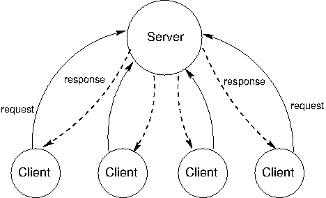
4.5.2   Client/Server Architecture

The client/server architecture is a way to dispense a service from a central source. A server provides a service and multiple clients communicate with the server to consume that service. In this architecture, clients and servers have different roles. The server's role is to respond to service requests from clients, while a client's role is to issue requests and make use of the server's response in order to perform some task. The diagram below illustrates the architecture.

The most influential use of the model is the modern World Wide Web. When a web browser displays the contents of a web page, several programs running on independent computers interact using the client/server architecture. This section describes the process of requesting a web page in order to illustrate central ideas in client/server distributed systems.

Roles. The web browser application on a Web user's computer has the role of the client when requesting a web page. When requesting the content from a domain name on the Internet, such as www.nytimes.com, it must communicate with at least two different servers.

The client first requests the Internet Protocol (IP) address of the computer located at that name from a Domain Name Server (DNS). A DNS provides the service of mapping domain names to IP addresses, which are numerical identifiers of machines on the Internet. Python can make such a request directly using the socket module.

>>> from socket import gethostbyname
>>> gethostbyname('www.nytimes.com')
'170.149.172.130'

The client then requests the contents of the web page from the web server located at that IP address. The response in this case is an HTML document that contains headlines and article excerpts of the day's news, as well as expressions that indicate how the web browser client should lay out that contents on the user's screen. Python can make the two requests required to retrieve this content using the urllib.request module.

>>> from urllib.request import urlopen
>>> response = urlopen('http://www.nytimes.com').read()
>>> response[:15]
b'<!DOCTYPE html>'

Upon receiving this response, the browser issues additional requests for images, videos, and other auxiliary components of the page. These requests are initiated because the original HTML document contains addresses of additional content and a description of how they embed into the page.

An HTTP Request. The Hypertext Transfer Protocol (HTTP) is a protocol implemented using TCP that governs communication for the World Wide Web (WWW). It assumes a client/server architecture between a web browser and a web server. HTTP specifies the format of messages exchanged between browsers and servers. All web browsers use the HTTP format to request pages from a web server, and all web servers use the HTTP format to send back their responses.

HTTP requests have several types, the most common of which is a GET request for a specific web page. A GET request specifies a location. For instance, typing the address http://en.wikipedia.org/wiki/UC_Berkeley into a web browser issues an HTTP GET request to port 80 of the web server at en.wikipedia.org for the contents at location /wiki/UC_Berkeley.

The server sends back an HTTP response:

HTTP/1.1 200 OK
Date: Mon, 23 May 2011 22:38:34 GMT
Server: Apache/1.3.3.7 (Unix) (Red-Hat/Linux)
Last-Modified: Wed, 08 Jan 2011 23:11:55 GMT
Content-Type: text/html; charset=UTF-8

... web page content ...

On the first line, the text 200 OK indicates that there were no errors in responding to the request. The subsequent lines of the header give information about the server, the date, and the type of content being sent back.

If you have typed in a wrong web address, or clicked on a broken link, you may have seen a message such as this error:

404 Error File Not Found

It means that the server sent back an HTTP header that started:

HTTP/1.1 404 Not Found

The numbers 200 and 404 are HTTP response codes. A fixed set of response codes is a common feature of a message protocol. Designers of protocols attempt to anticipate common messages that will be sent via the protocol and assign fixed codes to reduce transmission size and establish a common message semantics. In the HTTP protocol, the 200 response code indicates success, while 404 indicates an error that a resource was not found. A variety of other response codes exist in the HTTP 1.1 standard as well.

Modularity. The concepts of client and server are powerful abstractions. A server provides a service, possibly to multiple clients simultaneously, and a client consumes that service. The clients do not need to know the details of how the service is provided, or how the data they are receiving is stored or calculated, and the server does not need to know how its responses are going to be used.

On the web, we think of clients and servers as being on different machines, but even systems on a single machine can have client/server architectures. For example, signals from input devices on a computer need to be generally available to programs running on the computer. The programs are clients, consuming mouse and keyboard input data. The operating system's device drivers are the servers, taking in physical signals and serving them up as usable input. In addition, the central processing unit (CPU) and the specialized graphical processing unit (GPU) often participate in a client/server architecture with the CPU as the client and the GPU as a server of images.

A drawback of client/server systems is that the server is a single point of failure. It is the only component with the ability to dispense the service. There can be any number of clients, which are interchangeable and can come and go as necessary.

Another drawback of client-server systems is that computing resources become scarce if there are too many clients. Clients increase the demand on the system without contributing any computing resources.

4.5.3   Peer-to-Peer Systems

The client/server model is appropriate for service-oriented situations. However, there are other computational goals for which a more equal division of labor is a better choice. The term peer-to-peer is used to describe distributed systems in which labor is divided among all the components of the system. All the computers send and receive data, and they all contribute some processing power and memory. As a distributed system increases in size, its capacity of computational resources increases. In a peer-to-peer system, all components of the system contribute some processing power and memory to a distributed computation.

Division of labor among all participants is the identifying characteristic of a peer-to-peer system. This means that peers need to be able to communicate with each other reliably. In order to make sure that messages reach their intended destinations, peer-to-peer systems need to have an organized network structure. The components in these systems cooperate to maintain enough information about the locations of other components to send messages to intended destinations.

In some peer-to-peer systems, the job of maintaining the health of the network is taken on by a set of specialized components. Such systems are not pure peer-to-peer systems, because they have different types of components that serve different functions. The components that support a peer-to-peer network act like scaffolding: they help the network stay connected, they maintain information about the locations of different computers, and they help newcomers take their place within their neighborhood.

The most common applications of peer-to-peer systems are data transfer and data storage. For data transfer, each computer in the system contributes to send data over the network. If the destination computer is in a particular computer's neighborhood, that computer helps send data along. For data storage, the data set may be too large to fit on any single computer, or too valuable to store on just a single computer. Each computer stores a small portion of the data, and there may be multiple copies of the same data spread over different computers. When a computer fails, the data that was on it can be restored from other copies and put back when a replacement arrives.

Skype, the voice- and video-chat service, is an example of a data transfer application with a peer-to-peer architecture. When two people on different computers are having a Skype conversation, their communications are transmitted through a peer-to-peer network. This network is composed of other computers running the Skype application. Each computer knows the location of a few other computers in its neighborhood. A computer helps send a packet to its destination by passing it on a neighbor, which passes it on to some other neighbor, and so on, until the packet reaches its intended destination. Skype is not a pure peer-to-peer system. A scaffolding network of supernodes is responsible for logging-in and logging-out users, maintaining information about the locations of their computers, and modifying the network structure when users enter and exit.

4.6.1   MapReduce

The MapReduce framework assumes as input a large, unordered stream of input values of an arbitrary type. For instance, each input may be a line of text in some vast corpus. Computation proceeds in three steps.

1. A map function is applied to each input, which outputs zero or more intermediate key-value pairs of an arbitrary type.
2. All intermediate key-value pairs are grouped by key, so that pairs with the same key can be reduced together.
3. A reduce function combines the values for a given key k; it outputs zero or more values, which are each associated with k in the final output.

To perform this computation, the MapReduce framework creates tasks (perhaps on different machines) that perform various roles in the computation. A map task applies the map function to some subset of the input data and outputs intermediate key-value pairs. A reduce task sorts and groups key-value pairs by key, then applies the reduce function to the values for each key. All communication between map and reduce tasks is handled by the framework, as is the task of grouping intermediate key-value pairs by key.

In order to utilize multiple machines in a MapReduce application, multiple mappers run in parallel in a map phase, and multiple reducers run in parallel in a reduce phase. In between these phases, the sort phase groups together key-value pairs by sorting them, so that all key-value pairs with the same key are adjacent.

Consider the problem of counting the vowels in a corpus of text. We can solve this problem using the MapReduce framework with an appropriate choice of map and reduce functions. The map function takes as input a line of text and outputs key-value pairs in which the key is a vowel and the value is a count. Zero counts are omitted from the output:

def count_vowels(line):
    """A map function that counts the vowels in a line."""
    for vowel in 'aeiou':
        count = line.count(vowel)
        if count > 0:
            emit(vowel, count)

The reduce function is the built-in sum functions in Python, which takes as input an iterator over values (all values for a given key) and returns their sum.

4.6.2   Local Implementation

To specify a MapReduce application, we require an implementation of the MapReduce framework into which we can insert map and reduce functions. In the following section, we will use the open-source Hadoop implementation. In this section, we develop a minimal implementation using built-in tools of the Unix operating system.

The Unix operating system creates an abstraction barrier between user programs and the underlying hardware of a computer. It provides a mechanism for programs to communicate with each other, in particular by allowing one program to consume the output of another. In their seminal text on Unix programming, Kernigham and Pike assert that, ""The power of a system comes more from the relationships among programs than from the programs themselves."

A Python source file can be converted into a Unix program by adding a comment to the first line indicating that the program should be executed using the Python 3 interpreter. The input to a Unix program is an iterable object called standard input and accessed as sys.stdin. Iterating over this object yields string-valued lines of text. The output of a Unix program is called standard output and accessed as sys.stdout. The built-in print function writes a line of text to standard output. The following Unix program writes each line of its input to its output, in reverse:

#!/usr/bin/env python3

import sys

for line in sys.stdin:
    print(line.strip('\n')[::-1])

If we save this program to a file called rev.py, we can execute it as a Unix program. First, we need to tell the operating system that we have created an executable program:

$ chmod u+x rev.py

Next, we can pass input into this program. Input to a program can come from another program. This effect is achieved using the | symbol (called "pipe") which channels the output of the program before the pipe into the program after the pipe. The program nslookup outputs the host name of an IP address (in this case for the New York Times):

$ nslookup 170.149.172.130 | ./rev.py
moc.semityn.www

The cat program outputs the contents of files. Thus, the rev.py program can be used to reverse the contents of the rev.py file:

$ cat rev.py | ./rev.py
3nohtyp vne/nib/rsu/!#

sys tropmi

:nidts.sys ni enil rof
)]1-::[)'n\'(pirts.enil(tnirp

These tools are enough for us to implement a basic MapReduce framework. This version has only a single map task and single reduce task, which are both Unix programs implemented in Python. We run an entire MapReduce application using the following command:

$ cat input | ./mapper.py | sort | ./reducer.py

The mapper.py and reducer.py programs must implement the map function and reduce function, along with some simple input and output behavior. For instance, in order to implement the vowel counting application described above, we would write the following count_vowels_mapper.py program:

#!/usr/bin/env python3

import sys
from mapreduce import emit

def count_vowels(line):
    """A map function that counts the vowels in a line."""
    for vowel in 'aeiou':
        count = line.count(vowel)
        if count > 0:
            emit(vowel, count)

for line in sys.stdin:
    count_vowels(line)

In addition, we would write the following sum_reducer.py program:

#!/usr/bin/env python3

import sys
from mapreduce import group_values_by_key, emit

for key, value_iterator in group_values_by_key(sys.stdin):
    emit(key, sum(value_iterator))

The mapreduce module is a companion module to this text that provides the functions emit to emit a key-value pair and group_values_by_key to group together values that have the same key. This module also includes an interface to the Hadoop distributed implementation of MapReduce.

Finally, assume that we have the following input file called haiku.txt:

Google MapReduce
Is a Big Data framework
For batch processing

Local execution using Unix pipes gives us the count of each vowel in the haiku:

$ cat haiku.txt | ./count_vowels_mapper.py | sort | ./sum_reducer.py
'a'   6
'e'   5
'i'   2
'o'   5
'u'   1

4.6.3   Distributed Implementation

Hadoop is the name of an open-source implementation of the MapReduce framework that executes MapReduce applications on a cluster of machines, distributing input data and computation for efficient parallel processing. Its streaming interface allows arbitrary Unix programs to define the map and reduce functions. In fact, our count_vowels_mapper.py and sum_reducer.py can be used directly with a Hadoop installation to compute vowel counts on large text corpora.

Hadoop offers several advantages over our simplistic local MapReduce implementation. The first is speed: map and reduce functions are applied in parallel using different tasks on different machines running simultaneously. The second is fault tolerance: when a task fails for any reason, its result can be recomputed by another task in order to complete the overall computation. The third is monitoring: the framework provides a user interface for tracking the progress of a MapReduce application.

In order to run the vowel counting application using the provided mapreduce.py module, install Hadoop, change the assignment statement of HADOOP to the root of your local installation, copy a collection of text files into the Hadoop distributed file system, and then run:

$ python3 mapreduce.py run count_vowels_mapper.py sum_reducer.py [input] [output]

where [input] and [output] are directories in the Hadoop file system.

For more information on the Hadoop streaming interface and use of the system, consult the Hadoop Streaming Documentation.

4.7.1   Parallelism in Python

Before we dive deeper into the details of parallelism, let us first explore Python's support for parallel computation. Python provides two means of parallel execution: threading and multiprocessing.

Threading. In threading, multiple "threads" of execution exist within a single interpreter. Each thread executes code independently from the others, though they share the same data. However, the CPython interpreter, the main implementation of Python, only interprets code in one thread at a time, switching between them in order to provide the illusion of parallelism. On the other hand, operations external to the interpreter, such as writing to a file or accessing the network, may run in parallel.

The threading module contains classes that enable threads to be created and synchronized. The following is a simple example of a multithreaded program:

>>> import threading
>>> def thread_hello():
        other = threading.Thread(target=thread_say_hello, args=())
        other.start()
        thread_say_hello()

>>> def thread_say_hello():
        print('hello from', threading.current_thread().name)

>>> thread_hello()
hello from Thread-1
hello from MainThread

The Thread constructor creates a new thread. It requires a target function that the new thread should run, as well as the arguments to that function. Calling start on a Thread object marks it ready to run. The current_thread function returns the Thread object associated with the current thread of execution.

In this example, the prints can happen in any order, since we haven't synchronized them in any way.

Multiprocessing. Python also supports multiprocessing, which allows a program to spawn multiple interpreters, or processes, each of which can run code independently. These processes do not generally share data, so any shared state must be communicated between processes. On the other hand, processes execute in parallel according to the level of parallelism provided by the underlying operating system and hardware. Thus, if the CPU has multiple processor cores, Python processes can truly run concurrently.

The multiprocessing module contains classes for creating and synchronizing processes. The following is the hello example using processes:

>>> import multiprocessing
>>> def process_hello():
        other = multiprocessing.Process(target=process_say_hello, args=())
        other.start()
        process_say_hello()

>>> def process_say_hello():
        print('hello from', multiprocessing.current_process().name)

>>> process_hello()
hello from MainProcess
>>> hello from Process-1

As this example demonstrates, many of the classes and functions in multiprocessing are analogous to those in threading. This example also demonstrates how lack of synchronization affects shared state, as the display can be considered shared state. Here, the interpreter prompt from the interactive process appears before the print output from the other process.

4.7.2   The Problem with Shared State

To further illustrate the problem with shared state, let's look at a simple example of a counter that is shared between two threads:

import threading
from time import sleep

counter = [0]

def increment():
    count = counter[0]
    sleep(0) # try to force a switch to the other thread
    counter[0] = count + 1

other = threading.Thread(target=increment, args=())
other.start()
increment()
print('count is now: ', counter[0])

In this program, two threads attempt to increment the same counter. The CPython interpreter can switch between threads at almost any time. Only the most basic operations are atomic, meaning that they appear to occur instantly, with no switch possible during their evaluation or execution. Incrementing a counter requires multiple basic operations: read the old value, add one to it, and write the new value. The interpreter can switch threads between any of these operations.

In order to show what happens when the interpreter switches threads at the wrong time, we have attempted to force a switch by sleeping for 0 seconds. When this code is run, the interpreter often does switch threads at the sleep call. This can result in the following sequence of operations:

Thread 0                    Thread 1
read counter[0]: 0
                            read counter[0]: 0
calculate 0 + 1: 1
write 1 -> counter[0]
                            calculate 0 + 1: 1
                            write 1 -> counter[0]

The end result is that the counter has a value of 1, even though it was incremented twice! Worse, the interpreter may only switch at the wrong time very rarely, making this difficult to debug. Even with the sleep call, this program sometimes produces a correct count of 2 and sometimes an incorrect count of 1.

This problem arises only in the presence of shared data that may be mutated by one thread while another thread accesses it. Such a conflict is called a race condition, and it is an example of a bug that only exists in the parallel world.

In order to avoid race conditions, shared data that may be mutated and accessed by multiple threads must be protected against concurrent access. For example, if we can ensure that thread 1 only accesses the counter after thread 0 finishes accessing it, or vice versa, we can guarantee that the right result is computed. We say that shared data is synchronized if it is protected from concurrent access. In the next few subsections, we will see multiple mechanisms providing synchronization.

4.7.3   When No Synchronization is Necessary

In some cases, access to shared data need not be synchronized, if concurrent access cannot result in incorrect behavior. The simplest example is read-only data. Since such data is never mutated, all threads will always read the same values regardless when they access the data.

In rare cases, shared data that is mutated may not require synchronization. However, understanding when this is the case requires a deep knowledge of how the interpreter and underlying software and hardware work. Consider the following example:

items = []
flag = []

def consume():
    while not flag:
        pass
    print('items is', items)

def produce():
    consumer = threading.Thread(target=consume, args=())
    consumer.start()
    for i in range(10):
        items.append(i)
    flag.append('go')

produce()

Here, the producer thread adds items to items, while the consumer waits until flag is non-empty. When the producer finishes adding items, it adds an element to flag, allowing the consumer to proceed.

In most Python implementations, this example will work correctly. However, a common optimization in other compilers and interpreters, and even the hardware itself, is to reorder operations within a single thread that do not depend on each other for data. In such a system, the statement flag.append('go') may be moved before the loop, since neither depends on the other for data. In general, you should avoid code like this unless you are certain that the underlying system won't reorder the relevant operations.

4.7.4   Synchronized Data Structures

The simplest means of synchronizing shared data is to use a data structure that provides synchronized operations. The queue module contains a Queue class that provides synchronized first in, first out access to data. The put method adds an item to the Queue, and the get method retrieves an item. The class itself ensures that these methods are synchronized, so items are not lost no matter how thread operations are interleaved. Here is a producer/consumer example that uses a Queue:

from queue import Queue

queue = Queue()

def synchronized_consume():
    while True:
        print('got an item:', queue.get())
        queue.task_done()

def synchronized_produce():
    consumer = threading.Thread(target=synchronized_consume, args=())
    consumer.daemon = True
    consumer.start()
    for i in range(10):
        queue.put(i)
    queue.join()

synchronized_produce()

There are a few changes to this code, in addition to the Queue and get and put calls. We have marked the consumer thread as a daemon, which means that the program will not wait for that thread to complete before exiting. This allows us to use an infinite loop in the consumer. However, we do need to ensure that the main thread exits, but only after all items have been consumed from the Queue. The consumer calls the task_done method to inform the Queue that it is done processing an item, and the main thread calls the join method, which waits until all items have been processed, ensuring that the program exits only after that is the case.

A more complex example that makes use of a Queue is a parallel web crawler that searches for dead links on a website. This crawler follows all links that are hosted by the same site, so it must process a number of URLs, continually adding new ones to a Queue and removing URLs for processing. By using a synchronized Queue, multiple threads can safely add to and remove from the data structure concurrently.

4.7.5   Locks

When a synchronized version of a particular data structure is not available, we have to provide our own synchronization. A lock is a basic mechanism to do so. It can be acquired by at most one thread, after which no other thread may acquire it until it is released by the thread that previously acquired it.

In Python, the threading module contains a Lock class to provide locking. A Lock has acquire and release methods to acquire and release the lock, and the class guarantees that only one thread at a time can acquire it. All other threads that attempt to acquire a lock while it is already being held are forced to wait until it is released.

For a lock to protect a particular set of data, all the threads need to be programmed to follow a rule: no thread will access any of the shared data unless it owns that particular lock. In effect, all the threads need to "wrap" their manipulation of the shared data in acquire and release calls for that lock.

In the parallel web crawler, a set is used to keep track of all URLs that have been encountered by any thread, so as to avoid processing a particular URL more than once (and potentially getting stuck in a cycle). However, Python does not provide a synchronized set, so we must use a lock to protect access to a normal set:

seen = set()
seen_lock = threading.Lock()

def already_seen(item):
    seen_lock.acquire()
    result = True
    if item not in seen:
        seen.add(item)
        result = False
    seen_lock.release()
    return result

A lock is necessary here, in order to prevent another thread from adding the URL to the set between this thread checking if it is in the set and adding it to the set. Furthermore, adding to a set is not atomic, so concurrent attempts to add to a set may corrupt its internal data.

In this code, we had to be careful not to return until after we released the lock. In general, we have to ensure that we release a lock when we no longer need it. This can be very error-prone, particularly in the presence of exceptions, so Python provides a with compound statement that handles acquiring and releasing a lock for us:

def already_seen(item):
    with seen_lock:
        if item not in seen:
            seen.add(item)
            return False
        return True

The with statement ensures that seen_lock is acquired before its suite is executed and that it is released when the suite is exited for any reason. (The with statement can actually be used for operations other than locking, though we won't cover alternative uses here.)

Operations that must be synchronized with each other must use the same lock. However, two disjoint sets of operations that must be synchronized only with operations in the same set should use two different lock objects to avoid over-synchronization.

4.7.6   Barriers

Another way to avoid conflicting access to shared data is to divide a program into phases, ensuring that shared data is mutated in a phase in which no other thread accesses it. A barrier divides a program into phases by requiring all threads to reach it before any of them can proceed. Code that is executed after a barrier cannot be concurrent with code executed before the barrier.

In Python, the threading module provides a barrier in the form of the the wait method of a Barrier instance:

counters = [0, 0]
barrier = threading.Barrier(2)

def count(thread_num, steps):
    for i in range(steps):
        other = counters[1 - thread_num]
        barrier.wait() # wait for reads to complete
        counters[thread_num] = other + 1
        barrier.wait() # wait for writes to complete

def threaded_count(steps):
    other = threading.Thread(target=count, args=(1, steps))
    other.start()
    count(0, steps)
    print('counters:', counters)

threaded_count(10)

In this example, reading and writing to shared data take place in different phases, separated by barriers. The writes occur in the same phase, but they are disjoint; this disjointness is necessary to avoid concurrent writes to the same data in the same phase. Since this code is properly synchronized, both counters will always be 10 at the end.

The multithreaded particle simulator uses a barrier in a similar fashion to synchronize access to shared data. In the simulation, each thread owns a number of particles, all of which interact with each other over the course of many discrete timesteps. A particle has a position, velocity, and acceleration, and a new acceleration is computed in each timestep based on the positions of the other particles. The velocity of the particle must be updated accordingly, and its position according to its velocity.

As with the simple example above, there is a read phase, in which all particles' positions are read by all threads. Each thread updates its own particles' acceleration in this phase, but since these are disjoint writes, they need not be synchronized. In the write phase, each thread updates its own particles' velocities and positions. Again, these are disjoint writes, and they are protected from the read phase by barriers.

4.7.7   Message Passing

A final mechanism to avoid improper mutation of shared data is to entirely avoid concurrent access to the same data. In Python, using multiprocessing rather than threading naturally results in this, since processes run in separate interpreters with their own data. Any state required by multiple processes can be communicated by passing messages between processes.

The Pipe class in the multiprocessing module provides a communication channel between processes. By default, it is duplex, meaning a two-way channel, though passing in the argument False results in a one-way channel. The send method sends an object over the channel, while the recv method receives an object. The latter is blocking, meaning that a process that calls recv will wait until an object is received.

The following is a producer/consumer example using processes and pipes:

def process_consume(in_pipe):
    while True:
        item = in_pipe.recv()
        if item is None:
            return
        print('got an item:', item)

def process_produce():
    pipe = multiprocessing.Pipe(False)
    consumer = multiprocessing.Process(target=process_consume, args=(pipe[0],))
    consumer.start()
    for i in range(10):
        pipe[1].send(i)
    pipe[1].send(None) # done signal

process_produce()

In this example, we use a None message to signal the end of communication. We also passed in one end of the pipe as an argument to the target function when creating the consumer process. This is necessary, since state must be explicitly shared between processes.

The multiprocess version of the particle simulator uses pipes to communicate particle positions between processes in each timestep. In fact, it uses pipes to set up an entire circular pipeline between processes, in order to minimize communication. Each process injects its own particles' positions into its pipeline stage, which eventually go through a full rotation of the pipeline. At each step of the rotation, a process applies forces from the positions that are currently in its own pipeline stage on to its own particles, so that after a full rotation, all forces have been applied to its particles.

The multiprocessing module provides other synchronization mechanisms for processes, including synchronized queues, locks, and as of Python 3.3, barriers. For example, a lock or a barrier can be used to synchronize printing to the screen, avoiding the improper display output we saw previously.

4.7.8   Synchronization Pitfalls

While synchronization methods are effective for protecting shared state, they can also be used incorrectly, failing to accomplish the proper synchronization, over-synchronizing, or causing the program to hang as a result of deadlock.

Under-synchronization. A common pitfall in parallel computing is to neglect to properly synchronize shared accesses. In the set example, we need to synchronize the membership check and insertion together, so that another thread cannot perform an insertion in between these two operations. Failing to synchronize the two operations together is erroneous, even if they are separately synchronized.

Over-synchronization. Another common error is to over-synchronize a program, so that non-conflicting operations cannot occur concurrently. As a trivial example, we can avoid all conflicting access to shared data by acquiring a master lock when a thread starts and only releasing it when a thread completes. This serializes our entire code, so that nothing runs in parallel. In some cases, this can even cause our program to hang indefinitely. For example, consider a consumer/producer program in which the consumer obtains the lock and never releases it. This prevents the producer from producing any items, which in turn prevents the consumer from doing anything since it has nothing to consume.

While this example is trivial, in practice, programmers often over-synchronize their code to some degree, preventing their code from taking complete advantage of the available parallelism.

Deadlock. Because they cause threads or processes to wait on each other, synchronization mechanisms are vulnerable to deadlock, a situation in which two or more threads or processes are stuck, waiting for each other to finish. We have just seen how neglecting to release a lock can cause a thread to get stuck indefinitely. But even if threads or processes do properly release locks, programs can still reach deadlock.

The source of deadlock is a circular wait, illustrated below with processes. No process can continue because it is waiting for other processes that are waiting for it to complete.

As an example, we will set up a deadlock with two processes. Suppose they share a duplex pipe and attempt to communicate with each other as follows:

def deadlock(in_pipe, out_pipe):
    item = in_pipe.recv()
    print('got an item:', item)
    out_pipe.send(item + 1)

def create_deadlock():
    pipe = multiprocessing.Pipe()
    other = multiprocessing.Process(target=deadlock, args=(pipe[0], pipe[1]))
    other.start()
    deadlock(pipe[1], pipe[0])

create_deadlock()

Both processes attempt to receive data first. Recall that the recv method blocks until an item is available. Since neither process has sent anything, both will wait indefinitely for the other to send it data, resulting in deadlock.

Synchronization operations must be properly aligned to avoid deadlock. This may require sending over a pipe before receiving, acquiring multiple locks in the same order, and ensuring that all threads reach the right barrier at the right time.

4.7.9   Conclusion

As we have seen, parallelism presents new challenges in writing correct and efficient code. As the trend of increasing parallelism at the hardware level will continue for the foreseeable future, parallel computation will become more and more important in application programming. There is a very active body of research on making parallelism easier and less error-prone for programmers. Our discussion here serves only as a basic introduction to this crucial area of computer science.