Chapter 1: Building Abstractions with Functions
Contents
1.1 Introduction
Computer science is a tremendously broad academic discipline. The areas of globally distributed systems, artificial intelligence, robotics, graphics, security, scientific computing, computer architecture, and dozens of emerging sub-fields each expand with new techniques and discoveries every year. The rapid progress of computer science has left few aspects of human life unaffected. Commerce, communication, science, art, leisure, and politics have all been reinvented as computational domains.
The tremendous productivity of computer science is only possible because it is built upon an elegant and powerful set of fundamental ideas. All computing begins with representing information, specifying logic to process it, and designing abstractions that manage the complexity of that logic. Mastering these fundamentals will require us to understand precisely how computers interpret computer programs and carry out computational processes.
These fundamental ideas have long been taught at Berkeley using the classic textbook Structure and Interpretation of Computer Programs (SICP) by Harold Abelson and Gerald Jay Sussman with Julie Sussman. These lecture notes borrow heavily from that textbook, which the original authors have kindly licensed for adaptation and reuse.
The embarkment of our intellectual journey requires no revision, nor should we expect that it ever will.
We are about to study the idea of a computational process. Computational processes are abstract beings that inhabit computers. As they evolve, processes manipulate other abstract things called data. The evolution of a process is directed by a pattern of rules called a program. People create programs to direct processes. In effect, we conjure the spirits of the computer with our spells.
The programs we use to conjure processes are like a sorcerer's spells. They are carefully composed from symbolic expressions in arcane and esoteric programming languages that prescribe the tasks we want our processes to perform.
A computational process, in a correctly working computer, executes programs precisely and accurately. Thus, like the sorcerer's apprentice, novice programmers must learn to understand and to anticipate the consequences of their conjuring.
—Abelson and Sussman, SICP (1993)
1.1.1 Programming in Python
A language isn’t something you learn so much as something you join.
In order to define computational processes, we need a programming language; preferably one many humans and a great variety of computers can all understand. In this course, we will learn the Python language.
Python is a widely used programming language that has recruited enthusiasts from many professions: web programmers, game engineers, scientists, academics, and even designers of new programming languages. When you learn Python, you join a million-person-strong community of developers. Developer communities are tremendously important institutions: members help each other solve problems, share their code and experiences, and collectively develop software and tools. Dedicated members often achieve celebrity and widespread esteem for their contributions. Perhaps someday you will be named among these elite Pythonistas.
The Python language itself is the product of a large volunteer community that prides itself on the diversity of its contributors. The language was conceived and first implemented by Guido van Rossum in the late 1980's. The first chapter of his Python 3 Tutorial explains why Python is so popular, among the many languages available today.
Python excels as an instructional language because, throughout its history, Python's developers have emphasized the human interpretability of Python code, reinforced by the Zen of Python guiding principles of beauty, simplicity, and readability. Python is particularly appropriate for this course because its broad set of features support a variety of different programming styles, which we will explore. While there is no single way to program in Python, there are a set of conventions shared across the developer community that facilitate the process of reading, understanding, and extending existing programs. Hence, Python's combination of great flexibility and accessibility allows students to explore many programming paradigms, and then apply their newly acquired knowledge to thousands of ongoing projects.
These notes maintain the spirit of SICP by introducing the features of Python in lock step with techniques for abstraction design and a rigorous model of computation. In addition, these notes provide a practical introduction to Python programming, including some advanced language features and illustrative examples. Learning Python will come naturally as you progress through the course.
However, Python is a rich language with many features and uses, and we consciously introduce them slowly as we layer on fundamental computer science concepts. For experienced students who want to inhale all of the details of the language quickly, we recommend reading Mark Pilgrim's book Dive Into Python 3, which is freely available online. The topics in that book differ substantially from the topics of this course, but the book contains very valuable practical information on using the Python language. Be forewarned: unlike these notes, Dive Into Python 3 assumes substantial programming experience.
The best way to get started programming in Python is to interact with the interpreter directly. This section describes how to install Python 3, initiate an interactive session with the interpreter, and start programming.
1.1.2 Installing Python 3
As with all great software, Python has many versions. This course will use the most recent stable version of Python 3 (currently Python 3.2). Many computers have older versions of Python installed already, but those will not suffice for this course. You should be able to use any computer for this course, but expect to install Python 3. Don't worry, Python is free.
Dive Into Python 3 has detailed installation instructions for all major platforms. These instructions mention Python 3.1 several times, but you're better off with Python 3.2 (although the differences are insignificant for this course). All instructional machines in the EECS department have Python 3.2 already installed.
1.1.3 Interactive Sessions
In an interactive Python session, you type some Python code after the prompt, >>>. The Python interpreter reads and evaluates what you type, carrying out your various commands.
There are several ways to start an interactive session, and they differ in their properties. Try them all to find out what you prefer. They all use exactly the same interpreter behind the scenes.
- The simplest and most common way is to run the Python 3 application. Type python3 at a terminal prompt (Mac/Unix/Linux) or open the Python 3 application in Windows.
- A more user-friendly application for those learning the language is called Idle 3 (idle3). Idle colorizes your code (called syntax highlighting), pops up usage hints, and marks the source of some errors. Idle is always bundled with Python, so you have already installed it.
- The Emacs editor can run an interactive session inside one of its buffers. While slightly more challenging to learn, Emacs is a powerful and versatile editor for any programming language. Read the 61A Emacs Tutorial to get started. Many programmers who invest the time to learn Emacs never switch editors again.
In any case, if you see the Python prompt, >>>, then you have successfully started an interactive session. These notes depict example interactions using the prompt, followed by some input.
>>> 2 + 2
4
Controls: Each session keeps a history of what you have typed. To access that history, press <Control>-P (previous) and <Control>-N (next). <Control>-D exits a session, which discards this history.
1.1.4 First Example
And, as imagination bodies forthThe forms of things to unknown, and the poet's penTurns them to shapes, and gives to airy nothingA local habitation and a name.—William Shakespeare, A Midsummer-Night's Dream
To give Python the introduction it deserves, we will begin with an example that uses several language features. In the next section, we will have to start from scratch and build up the language piece by piece. Think of this section as a sneak preview of powerful features to come.
Python has built-in support for a wide range of common programming activities, like manipulating text, displaying graphics, and communicating over the Internet. The import statement
>>> from urllib.request import urlopen
loads functionality for accessing data on the Internet. In particular, it makes available a function called urlopen, which can access the content at a uniform resource locator (URL), which is a location of something on the Internet.
Statements & Expressions. Python code consists of statements and expressions. Broadly, computer programs consist of instructions to either
- Compute some value
- Carry out some action
Statements typically describe actions. When the Python interpreter executes a statement, it carries out the corresponding action. On the other hand, expressions typically describe computations that yield values. When Python evaluates an expression, it computes its value. This chapter introduces several types of statements and expressions.
The assignment statement
>>> shakespeare = urlopen('http://inst.eecs.berkeley.edu/~cs61a/fa11/shakespeare.txt')
associates the name shakespeare with the value of the expression that follows. That expression applies the urlopen function to a URL that contains the complete text of William Shakespeare's 37 plays, all in a single text document.
Functions. Functions encapsulate logic that manipulates data. A web address is a piece of data, and the text of Shakespeare's plays is another. The process by which the former leads to the latter may be complex, but we can apply that process using only a simple expression because that complexity is tucked away within a function. Functions are the primary topic of this chapter.
Another assignment statement
>>> words = set(shakespeare.read().decode().split())
associates the name words to the set of all unique words that appear in Shakespeare's plays, all 33,721 of them. The chain of commands to read, decode, and split, each operate on an intermediate computational entity: data is read from the opened URL, that data is decoded into text, and that text is split into words. All of those words are placed in a set.
Objects. A set is a type of object, one that supports set operations like computing intersections and testing membership. An object seamlessly bundles together data and the logic that manipulates that data, in a way that hides the complexity of both. Objects are the primary topic of Chapter 2.
The expression
>>> {w for w in words if len(w) >= 5 and w[::-1] in words}
{'madam', 'stink', 'leets', 'rever', 'drawer', 'stops', 'sessa',
'repaid', 'speed', 'redder', 'devil', 'minim', 'spots', 'asses',
'refer', 'lived', 'keels', 'diaper', 'sleek', 'steel', 'leper',
'level', 'deeps', 'repel', 'reward', 'knits'}
is a compound expression that evaluates to the set of Shakespearian words that appear both forward and in reverse. The cryptic notation w[::-1] enumerates each letter in a word, but the -1 says to step backwards (:: here means that the positions of the first and last characters to enumerate are defaulted.) When you enter an expression in an interactive session, Python prints its value on the following line, as shown.
Interpreters. Evaluating compound expressions requires a precise procedure that interprets code in a predictable way. A program that implements such a procedure, evaluating compound expressions and statements, is called an interpreter. The design and implementation of interpreters is the primary topic of Chapter 3.
When compared with other computer programs, interpreters for programming languages are unique in their generality. Python was not designed with Shakespeare or palindromes in mind. However, its great flexibility allowed us to process a large amount of text with only a few lines of code.
In the end, we will find that all of these core concepts are closely related: functions are objects, objects are functions, and interpreters are instances of both. However, developing a clear understanding of each of these concepts and their role in organizing code is critical to mastering the art of programming.
1.1.5 Practical Guidance: Errors
Python is waiting for your command. You are encouraged to experiment with the language, even though you may not yet know its full vocabulary and structure. However, be prepared for errors. While computers are tremendously fast and flexible, they are also extremely rigid. The nature of computers is described in Stanford's introductory course as
The fundamental equation of computers is: computer = powerful + stupid
Computers are very powerful, looking at volumes of data very quickly. Computers can perform billions of operations per second, where each operation is pretty simple.
Computers are also shockingly stupid and fragile. The operations that they can do are extremely rigid, simple, and mechanical. The computer lacks anything like real insight .. it's nothing like the HAL 9000 from the movies. If nothing else, you should not be intimidated by the computer as if it's some sort of brain. It's very mechanical underneath it all.
Programming is about a person using their real insight to build something useful, constructed out of these teeny, simple little operations that the computer can do.
—Francisco Cai and Nick Parlante, Stanford CS101
The rigidity of computers will immediately become apparent as you experiment with the Python interpreter: even the smallest spelling and formatting changes will cause unexpected outputs and errors.
Learning to interpret errors and diagnose the cause of unexpected errors is called debugging. Some guiding principles of debugging are:
- Test incrementally: Every well-written program is composed of small, modular components that can be tested individually. Test everything you write as soon as possible to catch errors early and gain confidence in your components.
- Isolate errors: An error in the output of a compound program, expression, or statement can typically be attributed to a particular modular component. When trying to diagnose a problem, trace the error to the smallest fragment of code you can before trying to correct it.
- Check your assumptions: Interpreters do carry out your instructions to the letter --- no more and no less. Their output is unexpected when the behavior of some code does not match what the programmer believes (or assumes) that behavior to be. Know your assumptions, then focus your debugging effort on verifying that your assumptions actually hold.
- Consult others: You are not alone! If you don't understand an error message, ask a friend, instructor, or search engine. If you have isolated an error, but can't figure out how to correct it, ask someone else to take a look. A lot of valuable programming knowledge is shared in the context of team problem solving.
Incremental testing, modular design, precise assumptions, and teamwork are themes that persist throughout this course. Hopefully, they will also persist throughout your computer science career.
1.2 The Elements of Programming
A programming language is more than just a means for instructing a computer to perform tasks. The language also serves as a framework within which we organize our ideas about processes. Programs serve to communicate those ideas among the members of a programming community. Thus, programs must be written for people to read, and only incidentally for machines to execute.
When we describe a language, we should pay particular attention to the means that the language provides for combining simple ideas to form more complex ideas. Every powerful language has three mechanisms for accomplishing this:
- primitive expressions and statements, which represent the simplest building blocks that the language provides,
- means of combination, by which compound elements are built from simpler ones, and
- means of abstraction, by which compound elements can be named and manipulated as units.
In programming, we deal with two kinds of elements: functions and data. (Soon we will discover that they are really not so distinct.) Informally, data is stuff that we want to manipulate, and functions describe the rules for manipulating the data. Thus, any powerful programming language should be able to describe primitive data and primitive functions and should have methods for combining and abstracting both functions and data.
1.2.1 Expressions
Having experimented with the full Python interpreter, we now must start anew, methodically developing the Python language piece by piece. Be patient if the examples seem simplistic --- more exciting material is soon to come.
We begin with primitive expressions. One kind of primitive expression is a number. More precisely, the expression that you type consists of the numerals that represent the number in base 10.
>>> 42
42
Expressions representing numbers may be combined with mathematical operators to form a compound expression, which the interpreter will evaluate:
>>> -1 - -1
0
>>> 1/2 + 1/4 + 1/8 + 1/16 + 1/32 + 1/64 + 1/128
0.9921875
These mathematical expressions use infix notation, where the operator (e.g., +, -, *, or /) appears in between the operands (numbers). Python includes many ways to form compound expressions. Rather than attempt to enumerate them all immediately, we will introduce new expression forms as we go, along with the language features that they support.
1.2.2 Call Expressions
The most important kind of compound expression is a call expression, which applies a function to some arguments. Recall from algebra that the mathematical notion of a function is a mapping from some input arguments to an output value. For instance, the max function maps its inputs to a single output, which is the largest of the inputs. A function in Python is more than just an input-output mapping; it describes a computational process. However, the way in which Python expresses function application is the same as in mathematics.
>>> max(7.5, 9.5)
9.5
This call expression has subexpressions: the operator precedes parentheses, which enclose a comma-delimited list of operands. The operator must be a function. The operands can be any values; in this case they are numbers. When this call expression is evaluated, we say that the function max is called with arguments 7.5 and 9.5, and returns a value of 9.5.
The order of the arguments in a call expression matters. For instance, the function pow raises its first argument to the power of its second argument.
>>> pow(100, 2)
10000
>>> pow(2, 100)
1267650600228229401496703205376
Function notation has several advantages over the mathematical convention of infix notation. First, functions may take an arbitrary number of arguments:
>>> max(1, -2, 3, -4)
3
No ambiguity can arise, because the function name always precedes its arguments.
Second, function notation extends in a straightforward way to nested expressions, where the elements are themselves compound expressions. In nested call expressions, unlike compound infix expressions, the structure of the nesting is entirely explicit in the parentheses.
>>> max(min(1, -2), min(pow(3, 5), -4))
-2
There is no limit (in principle) to the depth of such nesting and to the overall complexity of the expressions that the Python interpreter can evaluate. However, humans quickly get confused by multi-level nesting. An important role for you as a programmer is to structure expressions so that they remain interpretable by yourself, your programming partners, and others who may read your code in the future.
Finally, mathematical notation has a great variety of forms: multiplication appears between terms, exponents appear as superscripts, division as a horizontal bar, and a square root as a roof with slanted siding. Some of this notation is very hard to type! However, all of this complexity can be unified via the notation of call expressions. While Python supports common mathematical operators using infix notation (like + and -), any operator can be expressed as a function with a name.
1.2.3 Importing Library Functions
Python defines a very large number of functions, including the operator functions mentioned in the preceding section, but does not make their names available by default, so as to avoid complete chaos. Instead, it organizes the functions and other quantities that it knows about into modules, which together comprise the Python Library. To use these elements, one imports them. For example, the math module provides a variety of familiar mathematical functions:
>>> from math import sqrt, exp
>>> sqrt(256)
16.0
>>> exp(1)
2.718281828459045
and the operator module provides access to functions corresponding to infix operators:
>>> from operator import add, sub, mul
>>> add(14, 28)
42
>>> sub(100, mul(7, add(8, 4)))
16
An import statement designates a module name (e.g., operator or math), and then lists the named attributes of that module to import (e.g., sqrt or exp).
The Python 3 Library Docs list the functions defined by each module, such as the math module. However, this documentation is written for developers who know the whole language well. For now, you may find that experimenting with a function tells you more about its behavior than reading the documemtation. As you become familiar with the Python language and vocabulary, this documentation will become a valuable reference source.
1.2.4 Names and the Environment
A critical aspect of a programming language is the means it provides for using names to refer to computational objects. If a value has been given a name, we say that the name binds to the value.
In Python, we can establish new bindings using the assignment statement, which contains a name to the left of = and a value to the right:
>>> radius = 10
>>> radius
10
>>> 2 * radius
20
Names are also bound via import statements.
>>> from math import pi
>>> pi * 71 / 223
1.0002380197528042
We can also assign multiple values to multiple names in a single statement, where names and expressions are separated by commas.
>>> area, circumference = pi * radius * radius, 2 * pi * radius
>>> area
314.1592653589793
>>> circumference
62.83185307179586
The = symbol is called the assignment operator in Python (and many other languages). Assignment is Python's simplest means of abstraction, for it allows us to use simple names to refer to the results of compound operations, such as the area computed above. In this way, complex programs are constructed by building, step by step, computational objects of increasing complexity.
The possibility of binding names to values and later retrieving those values by name means that the interpreter must maintain some sort of memory that keeps track of the names, values, and bindings. This memory is called an environment.
Names can also be bound to functions. For instance, the name max is bound to the max function we have been using. Functions, unlike numbers, are tricky to render as text, so Python prints an identifying description instead, when asked to print a function:
>>> max
<built-in function max>
We can use assignment statements to give new names to existing functions.
>>> f = max
>>> f
<built-in function max>
>>> f(3, 4)
4
And successive assignment statements can rebind a name to a new value.
>>> f = 2
>>> f
2
In Python, the names bound via assignment are often called variable names because they can be bound to a variety of different values in the course of executing a program.
1.2.5 Evaluating Nested Expressions
One of our goals in this chapter is to isolate issues about thinking procedurally. As a case in point, let us consider that, in evaluating nested call expressions, the interpreter is itself following a procedure.
To evaluate a call expression, Python will do the following:
- Evaluate the operator and operand subexpressions, then
- Apply the function that is the value of the operator subexpression to the arguments that are the values of the operand subexpressions.
Even this simple procedure illustrates some important points about processes in general. The first step dictates that in order to accomplish the evaluation process for a call expression we must first evaluate other expressions. Thus, the evaluation procedure is recursive in nature; that is, it includes, as one of its steps, the need to invoke the rule itself.
For example, evaluating
>>> mul(add(2, mul(4, 6)), add(3, 5))
208
requires that this evaluation procedure be applied four times. If we draw each expression that we evaluate, we can visualize the hierarchical structure of this process.
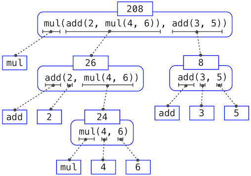
This illustration is called an expression tree. In computer science, trees grow from the top down. The objects at each point in a tree are called nodes; in this case, they are expressions paired with their values.
Evaluating its root, the full expression, requires first evaluating the branches that are its subexpressions. The leaf expressions (that is, nodes with no branches stemming from them) represent either functions or numbers. The interior nodes have two parts: the call expression to which our evaluation rule is applied, and the result of that expression. Viewing evaluation in terms of this tree, we can imagine that the values of the operands percolate upward, starting from the terminal nodes and then combining at higher and higher levels.
Next, observe that the repeated application of the first step brings us to the point where we need to evaluate, not call expressions, but primitive expressions such as numerals (e.g., 2) and names (e.g., add). We take care of the primitive cases by stipulating that
- A numeral evaluates to the number it names,
- A name evaluates to the value associated with that name in the current environment.
Notice the important role of an environment in determining the meaning of the symbols in expressions. In Python, it is meaningless to speak of the value of an expression such as
>>> add(x, 1)
without specifying any information about the environment that would provide a meaning for the name x (or even for the name add). Environments provide the context in which evaluation takes place, which plays an important role in our understanding of program execution.
This evaluation procedure does not suffice to evaluate all Python code, only call expressions, numerals, and names. For instance, it does not handle assignment statements. Executing
>>> x = 3
does not return a value nor evaluate a function on some arguments, since the purpose of assignment is instead to bind a name to a value. In general, statements are not evaluated but executed; they do not produce a value but instead make some change. Each type of statement or expression has its own evaluation or execution procedure, which we will introduce incrementally as we proceed.
A pedantic note: when we say that "a numeral evaluates to a number," we actually mean that the Python interpreter evaluates a numeral to a number. It is the interpreter which endows meaning to the programming language. Given that the interpreter is a fixed program that always behaves consistently, we can loosely say that numerals (and expressions) themselves evaluate to values in the context of Python programs.
1.2.6 Function Diagrams
As we continue to develop a formal model of evaluation, we will find that diagramming the internal state of the interpreter helps us track the progress of our evaluation procedure. An essential part of these diagrams is a representation of a function.
Pure functions. Functions have some input (their arguments) and return some output (the result of applying them). The built-in function
>>> abs(-2)
2
can be depicted as a small machine that takes input and produces output.
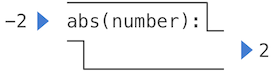
The function abs is pure. Pure functions have the property that applying them has no effects beyond returning a value.
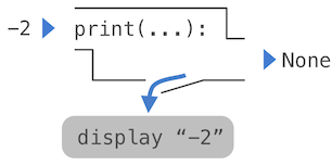
Non-pure functions. In addition to returning a value, applying a non-pure function can generate side effects, which make some change to the state of the interpreter or computer. A common side effect is to generate additional output beyond the return value, using the print function.
>>> print(-2)
-2
>>> print(1, 2, 3)
1 2 3
While print and abs may appear to be similar in these examples, they work in fundamentally different ways. The value that print returns is always None, a special Python value that represents nothing. The interactive Python interpreter does not automatically print the value None. In the case of print, the function itself is printing output as a side effect of being called.
A nested expression of calls to print highlights the non-pure character of the function.
>>> print(print(1), print(2))
1
2
None None
If you find this output to be unexpected, draw an expression tree to clarify why evaluating this expression produces this peculiar output.
Be careful with print! The fact that it returns None means that it should not be the expression in an assignment statement.
>>> two = print(2)
2
>>> print(two)
None
Signatures. Functions differ in the number of arguments that they are allowed to take. To track these requirements, we draw each function in a way that shows the function name and names of its arguments. The function abs takes only one argument called number; providing more or fewer will result in an error. The function print can take an arbitrary number of arguments, hence its rendering as print(...). A description of the arguments that a function can take is called the function's signature.
1.3 Defining New Functions
We have identified in Python some of the elements that must appear in any powerful programming language:
- Numbers and arithmetic operations are built-in data and functions.
- Nested function application provides a means of combining operations.
- Binding names to values provides a limited means of abstraction.
Now we will learn about function definitions, a much more powerful abstraction technique by which a name can be bound to compound operation, which can then be referred to as a unit.
We begin by examining how to express the idea of "squaring." We might say, "To square something, multiply it by itself." This is expressed in Python as
>>> def square(x):
        return mul(x, x)
which defines a new function that has been given the name square. This user-defined function is not built into the interpreter. It represents the compound operation of multiplying something by itself. The x in this definition is called a formal parameter, which provides a name for the thing to be multiplied. The definition creates this user-defined function and associates it with the name square.
Function definitions consist of a def statement that indicates a <name> and a list of named <formal parameters>, then a return statement, called the function body, that specifies the <return expression> of the function, which is an expression to be evaluated whenever the function is applied.
- def <name>(<formal parameters>):
- return <return expression>
The second line must be indented! Convention dictates that we indent with four spaces, rather than a tab. The return expression is not evaluated right away; it is stored as part of the newly defined function and evaluated only when the function is eventually applied. (Soon, we will see that the indented region can span multiple lines.)
Having defined square, we can apply it with a call expression:
>>> square(21)
441
>>> square(add(2, 5))
49
>>> square(square(3))
81
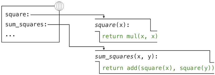
We can also use square as a building block in defining other functions. For example, we can easily define a function sum_squares that, given any two numbers as arguments, returns the sum of their squares:
>>> def sum_squares(x, y):
        return add(square(x), square(y))
>>> sum_squares(3, 4)
25
User-defined functions are used in exactly the same way as built-in functions. Indeed, one cannot tell from the definition of sum_squares whether square is built into the interpreter, imported from a module, or defined by the user.
1.3.1 Environments
Our subset of Python is now complex enough that the meaning of programs is non-obvious. What if a formal parameter has the same name as a built-in function? Can two functions share names without confusion? To resolve such questions, we must describe environments in more detail.
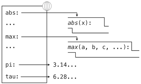
An environment in which an expression is evaluated consists of a sequence of frames, depicted as boxes. Each frame contains bindings, which associate a name with its corresponding value. There is a single global frame that contains name bindings for all built-in functions (only abs and max are shown). We indicate the global frame with a globe symbol.
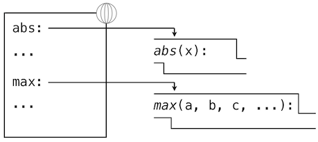
Assignment and import statements add entries to the first frame of the current environment. So far, our environment consists only of the global frame.
>>> from math import pi
>>> tau = 2 * pi
A def statement also binds a name to the function created by the definition. The resulting environment after defining square appears below:
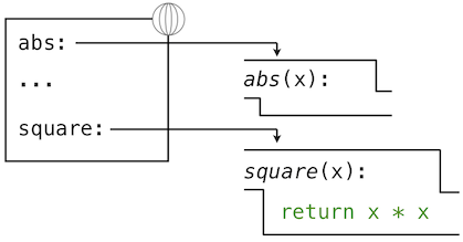
These environment diagrams show the bindings of the current environment, along with the values (which are not part of any frame) to which names are bound. Notice that the name of a function is repeated, once in the frame, and once as part of the function itself. This repetition is intentional: many different names may refer to the same function, but that function itself has only one intrinsic name. However, looking up the value for a name in an environment only inspects name bindings. The intrinsic name of a function does not play a role in looking up names. In the example we saw earlier,
>>> f = max
>>> f
<built-in function max>
The name max is the intrinsic name of the function, and that's what you see printed as the value for f. In addition, both the names max and f are bound to that same function in the global environment.
As we proceed to introduce additional features of Python, we will have to extend these diagrams. Every time we do, we will list the new features that our diagrams can express.
New environment Features: Assignment and user-defined function definition.
1.3.2 Calling User-Defined Functions
To evaluate a call expression whose operator names a user-defined function, the Python interpreter follows a process similar to the one for evaluating expressions with a built-in operator function. That is, the interpreter evaluates the operand expressions, and then applies the named function to the resulting arguments.
The act of applying a user-defined function introduces a second local frame, which is only accessible to that function. To apply a user-defined function to some arguments:
- Bind the arguments to the names of the function's formal parameters in a new local frame.
- Evaluate the body of the function in the environment beginning at that frame and ending at the global frame.
The environment in which the body is evaluated consists of two frames: first the local frame that contains argument bindings, then the global frame that contains everything else. Each instance of a function application has its own independent local frame.
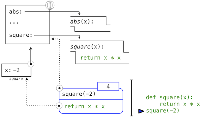
This figure includes two different aspects of the Python interpreter: the current environment, and a part of the expression tree related to the current line of code being evaluated. We have depicted the evaluation of a call expression that has a user-defined function (in blue) as a two-part rounded rectangle. Dotted arrows indicate which environment is used to evaluate the expression in each part.
- The top half shows the call expression being evaluated. This call expression is not internal to any function, so it is evaluated in the global environment. Thus, any names within it (such as square) are looked up in the global frame.
- The bottom half shows the body of the square function. Its return expression is evaluated in the new environment introduced by step 1 above, which binds the name of square's formal parameter x to the value of its argument, -2.
The order of frames in an environment affects the value returned by looking up a name in an expression. We stated previously that a name is evaluated to the value associated with that name in the current environment. We can now be more precise:
- A name evaluates to the value bound to that name in the earliest frame of the current environment in which that name is found.
Our conceptual framework of environments, names, and functions constitutes a model of evaluation; while some mechanical details are still unspecified (e.g., how a binding is implemented), our model does precisely and correctly describe how the interpreter evaluates call expressions. In Chapter 3 we shall see how this model can serve as a blueprint for implementing a working interpreter for a programming language.
New environment Feature: Function application.
1.3.3 Example: Calling a User-Defined Function
Let us again consider our two simple definitions:
>>> from operator import add, mul
>>> def square(x):
        return mul(x, x)
>>> def sum_squares(x, y):
        return add(square(x), square(y))
And the process that evaluates the following call expression:
>>> sum_squares(5, 12)
169
Python first evaluates the name sum_squares, which is bound to a user-defined function in the global frame. The primitive numeric expressions 5 and 12 evaluate to the numbers they represent.
Next, Python applies sum_squares, which introduces a local frame that binds x to 5 and y to 12.
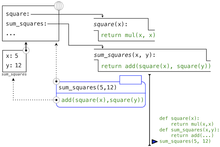
In this diagram, the local frame points to its successor, the global frame. All local frames must point to a predecessor, and these links define the sequence of frames that is the current environment.
The body of sum_squares contains this call expression:
   add     (  square(x)  ,  square(y)  )
 ________     _________     _________
"operator"   "operand 0"   "operand 1"
All three subexpressions are evalauted in the current environment, which begins with the frame labeled sum_squares. The operator subexpression add is a name found in the global frame, bound to the built-in function for addition. The two operand subexpressions must be evaluated in turn, before addition is applied. Both operands are evaluated in the current environment beginning with the frame labeled sum_squares. In the following environment diagrams, we will call this frame A and replace arrows pointing to this frame with the label A as well.
In operand 0, square names a user-defined function in the global frame, while x names the number 5 in the local frame. Python applies square to 5 by introducing yet another local frame that binds x to 5.
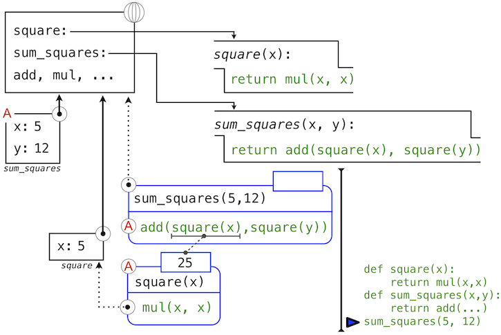
Using this local frame, the body expression mul(x, x) evaluates to 25.
Our evaluation procedure now turns to operand 1, for which y names the number 12. Python evaluates the body of square again, this time introducing yet another local environment frame that binds x to 12. Hence, operand 1 evaluates to 144.
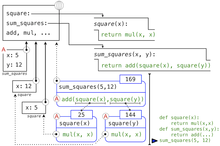
Finally, applying addition to the arguments 25 and 144 yields a final value for the body of sum_squares: 169.
This figure, while complex, serves to illustrate many of the fundamental ideas we have developed so far. Names are bound to values, which spread across many local frames that all precede a single global frame that contains shared names. Expressions are tree-structured, and the environment must be augmented each time a subexpression contains a call to a user-defined function.
All of this machinery exists to ensure that names resolve to the correct values at the correct points in the expression tree. This example illustrates why our model requires the complexity that we have introduced. All three local frames contain a binding for the name x, but that name is bound to different values in different frames. Local frames keep these names separate.
1.3.4 Local Names
One detail of a function's implementation that should not affect the function's behavior is the implementer's choice of names for the function's formal parameters. Thus, the following functions should provide the same behavior:
>>> def square(x):
        return mul(x, x)
>>> def square(y):
        return mul(y, y)
This principle -- that the meaning of a function should be independent of the parameter names chosen by its author -- has important consequences for programming languages. The simplest consequence is that the parameter names of a function must remain local to the body of the function.
If the parameters were not local to the bodies of their respective functions, then the parameter x in square could be confused with the parameter x in sum_squares. Critically, this is not the case: the binding for x in different local frames are unrelated. Our model of computation is carefully designed to ensure this independence.
We say that the scope of a local name is limited to the body of the user-defined function that defines it. When a name is no longer accessible, it is out of scope. This scoping behavior isn't a new fact about our model; it is a consequence of the way environments work.
1.3.5 Practical Guidance: Choosing Names
The interchangeabily of names does not imply that formal parameter names do not matter at all. To the contrary, well-chosen function and parameter names are essential for the human interpretability of function definitions!
The following guidelines are adapted from the style guide for Python code, which serves as a guide for all (non-rebellious) Python programmers. A shared set of conventions smooths communication among members of a programming community. As a side effect of following these conventions, you will find that your code becomes more internally consistent.
- Function names should be lowercase, with words separated by underscores. Descriptive names are encouraged.
- Function names typically evoke operations applied to arguments by the interpreter (e.g., print, add, square) or the name of the quantity that results (e.g., max, abs, sum).
- Parameter names should be lowercase, with words separated by underscores. Single-word names are preferred.
- Parameter names should evoke the role of the parameter in the function, not just the type of value that is allowed.
- Single letter parameter names are acceptable when their role is obvious, but never use "l" (lowercase ell), "O" (capital oh), or "I" (capital i) to avoid confusion with numerals.
Review these guidelines periodically as you write programs, and soon your names will be delightfully Pythonic.
1.3.6 Functions as Abstractions
Though it is very simple, sum_squares exemplifies the most powerful property of user-defined functions. The function sum_squares is defined in terms of the function square, but relies only on the relationship that square defines between its input arguments and its output values.
We can write sum_squares without concerning ourselves with how to square a number. The details of how the square is computed can be suppressed, to be considered at a later time. Indeed, as far as sum_squares is concerned, square is not a particular function body, but rather an abstraction of a function, a so-called functional abstraction. At this level of abstraction, any function that computes the square is equally good.
Thus, considering only the values they return, the following two functions for squaring a number should be indistinguishable. Each takes a numerical argument and produces the square of that number as the value.
>>> def square(x):
        return mul(x, x)
>>> def square(x):
        return mul(x, x-1) + x
In other words, a function definition should be able to suppress details. The users of the function may not have written the function themselves, but may have obtained it from another programmer as a "black box". A user should not need to know how the function is implemented in order to use it. The Python Library has this property. Many developers use the functions defined there, but few ever inspect their implementation. In fact, many implementations of Python Library functions are not written in Python at all, but instead in the C language.
1.3.7 Operators
Mathematical operators (like + and -) provided our first example of a method of combination, but we have yet to define an evaluation procedure for expressions that contain these operators.
Python expressions with infix operators each have their own evaluation procedures, but you can often think of them as short-hand for call expressions. When you see
>>> 2 + 3
5
simply consider it to be short-hand for
>>> add(2, 3)
5
Infix notation can be nested, just like call expressions. Python applies the normal mathematical rules of operator precedence, which dictate how to interpret a compound expression with multiple operators.
>>> 2 + 3 * 4 + 5
19
evaluates to the same result as
>>> add(add(2, mul(3, 4)) , 5)
19
The nesting in the call expression is more explicit than the operator version. Python also allows subexpression grouping with parentheses, to override the normal precedence rules or make the nested structure of an expression more explicit.
>>> (2 + 3) * (4 + 5)
45
evaluates to the same result as
>>> mul(add(2, 3), add(4, 5))
45
You should feel free to use these operators and parentheses in your programs. Idiomatic Python prefers operators over call expressions for simple mathematical operations.
1.4 Practical Guidance: The Art of the Function
Functions are an essential ingredient of all programs, large and small, and serve as our primary medium to express computational processes in a programming language. So far, we have discussed the formal properties of functions and how they are applied. We now turn to the topic of what makes a good function. Fundamentally, the qualities of good functions all reinforce the idea that functions are abstractions.
- Each function should have exactly one job. That job should be identifiable with a short name and characterizable in a single line of text. Functions that perform multiple jobs in sequence should be divided into multiple functions.
- Don't repeat yourself is a central tenet of software engineering. The so-called DRY principle states that multiple fragments of code should not describe redundant logic. Instead, that logic should be implemented once, given a name, and applied multiple times. If you find yourself copying and pasting a block of code, you have probably found an opportunity for functional abstraction.
- Functions should be defined generally. Squaring is not in the Python Library precisely because it is a special case of the pow function, which raises numbers to arbitrary powers.
These guidelines improve the readability of code, reduce the number of errors, and often minimize the total amount of code written. Decomposing a complex task into concise functions is a skill that takes experience to master. Fortunately, Python provides several features to support your efforts.
1.4.1 Docstrings
A function definition will often include documentation describing the function, called a docstring, which must be indented along with the function body. Docstrings are conventionally triple quoted. The first line describes the job of the function in one line. The following lines can describe arguments and clarify the behavior of the function:
>>> def pressure(v, t, n):
        """Compute the pressure in pascals of an ideal gas.

        Applies the ideal gas law: http://en.wikipedia.org/wiki/Ideal_gas_law

        v -- volume of gas, in cubic meters
        t -- absolute temperature in degrees kelvin
        n -- particles of gas
        """
        k = 1.38e-23  # Boltzmann's constant
        return n * k * t / v
When you call help with the name of a function as an argument, you see its docstring (type q to quit Python help).
>>> help(pressure)
When writing Python programs, include docstrings for all but the simplest functions. Remember, code is written only once, but often read many times. The Python docs include docstring guidelines that maintain consistency across different Python projects.
1.4.2 Default Argument Values
A consequence of defining general functions is the introduction of additional arguments. Functions with many arguments can be awkward to call and difficult to read.
In Python, we can provide default values for the arguments of a function. When calling that function, arguments with default values are optional. If they are not provided, then the default value is bound to the formal parameter name instead. For instance, if an application commonly computes pressure for one mole of particles, this value can be provided as a default:
>>> k_b=1.38e-23  # Boltzmann's constant
>>> def pressure(v, t, n=6.022e23):
        """Compute the pressure in pascals of an ideal gas.

        v -- volume of gas, in cubic meters
        t -- absolute temperature in degrees kelvin
        n -- particles of gas (default: one mole)
        """
        return n * k_b * t / v
>>> pressure(1, 273.15)
2269.974834
Here, pressure is defined to take three arguments, but only two are provided in the call expression that follows. In this case, the value for n is taken from the def statement defaults (which looks like an assignment to n, although as this discussion suggests, it is more of a conditional assignment.)
As a guideline, most data values used in a function's body should be expressed as default values to named arguments, so that they are easy to inspect and can be changed by the function caller. Some values that never change, like the fundamental constant k_b, can be defined in the global frame.
1.5 Control
The expressive power of the functions that we can define at this point is very limited, because we have not introduced a way to make tests and to perform different operations depending on the result of a test. Control statements will give us this capacity. Control statements differ fundamentally from the expressions that we have studied so far. They deviate from the strict evaluation of subexpressions from left to write, and get their name from the fact that they control what the interpreter should do next, possibly based on the values of expressions.
1.5.1 Statements
So far, we have primarily considered how to evaluate expressions. However, we have seen three kinds of statements: assignment, def, and return statements. These lines of Python code are not themselves expressions, although they all contain expressions as components.
To emphasize that the value of a statement is irrelevant (or nonexistant), we describe statements as being executed rather than evaluated. Each statement describes some change to the interpreter state, and executing a statement applies that change. As we have seen for return and assignment statements, executing statements can involve evaluating subexpressions contained within them.
Expressions can also be executed as statements, in which case they are evaluated, but their value is discarded. Executing a pure function has no effect, but executing a non-pure function can cause effects as a consequence of function application.
Consider, for instance,
>>> def square(x):
        mul(x, x) # Watch out! This call doesn't return a value.
This is valid Python, but probably not what was intended. The body of the function consists of an expression. An expression by itself is a valid statement, but the effect of the statement is that the mul function is called, and the result is discarded. If you want to do something with the result of an expression, you need to say so: you might store it with an assignment statement, or return it with a return statement:
>>> def square(x):
        return mul(x, x)
Sometimes it does make sense to have a function whose body is an expression, when a non-pure function like print is called.
>>> def print_square(x):
        print(square(x))
At its highest level, the Python interpreter's job is to execute programs, composed of statements. However, much of the interesting work of computation comes from evaluating expressions. Statements govern the relationship among different expressions in a program and what happens to their results.
1.5.2 Compound Statements
In general, Python code is a sequence of statements. A simple statement is a single line that doesn't end in a colon. A compound statement is so called because it is composed of other statements (simple and compound). Compound statements typically span multiple lines and start with a one-line header ending in a colon, which identifies the type of statement. Together, a header and an indented suite of statements is called a clause. A compound statement consists of one or more clauses:
<header>:
    <statement>
    <statement>
    ...
<separating header>:
    <statement>
    <statement>
    ...
...
We can understand the statements we have already introduced in these terms.
- Expressions, return statements, and assignment statements are simple statements.
- A def statement is a compound statement. The suite that follows the def header defines the function body.
Specialized evaluation rules for each kind of header dictate when and if the statements in its suite are executed. We say that the header controls its suite. For example, in the case of def statements, we saw that the return expression is not evaluated immediately, but instead stored for later use when the defined function is eventually applied.
We can also understand multi-line programs now.
- To execute a sequence of statements, execute the first statement. If that statement does not redirect control, then proceed to execute the rest of the sequence of statements, if any remain.
This definition exposes the essential structure of a recursively defined sequence: a sequence can be decomposed into its first element and the rest of its elements. The "rest" of a sequence of statements is itself a sequence of statements! Thus, we can recursively apply this execution rule. This view of sequences as recursive data structures will appear again in later chapters.
The important consequence of this rule is that statements are executed in order, but later statements may never be reached, because of redirected control.
Practical Guidance. When indenting a suite, all lines must be indented the same amount and in the same way (spaces, not tabs). Any variation in indentation will cause an error.
1.5.3 Defining Functions II: Local Assignment
Originally, we stated that the body of a user-defined function consisted only of a return statement with a single return expression. In fact, functions can define a sequence of operations that extends beyond a single expression. The structure of compound Python statements naturally allows us to extend our concept of a function body to multiple statements.
Whenever a user-defined function is applied, the sequence of clauses in the suite of its definition is executed in a local environment. A return statement redirects control: the process of function application terminates whenever the first return statement is executed, and the value of the return expression is the returned value of the function being applied.
Thus, assignment statements can now appear within a function body. For instance, this function returns the absolute difference between two quantities as a percentage of the first, using a two-step calculation:
>>> def percent_difference(x, y):
        difference = abs(x-y)
        return 100 * difference / x
>>> percent_difference(40, 50)
25.0
The effect of an assignment statement is to bind a name to a value in the first frame of the current environment. As a consequence, assignment statements within a function body cannot affect the global frame. The fact that functions can only manipulate their local environment is critical to creating modular programs, in which pure functions interact only via the values they take and return.
Of course, the percent_difference function could be written as a single expression, as shown below, but the return expression is more complex.
>>> def percent_difference(x, y):
        return 100 * abs(x-y) / x
So far, local assignment hasn't increased the expressive power of our function definitions. It will do so, when combined with the control statements below. In addition, local assignment also plays a critical role in clarifying the meaning of complex expressions by assigning names to intermediate quantities.
New environment Feature: Local assignment.
1.5.4 Conditional Statements
Python has a built-in function for computing absolute values.
>>> abs(-2)
2
We would like to be able to implement such a function ourselves, but we cannot currently define a function that has a test and a choice. We would like to express that if x is positive, abs(x) returns x. Furthermore, if x is 0, abs(x) returns 0. Otherwise, abs(x) returns -x. In Python, we can express this choice with a conditional statement.
>>> def absolute_value(x):
        """Compute abs(x)."""
        if x > 0:
            return x
        elif x == 0:
            return 0
        else:
            return -x
>>> absolute_value(-2) == abs(-2)
True
This implementation of absolute_value raises several important issues.
Conditional statements. A conditional statement in Python consist of a series of headers and suites: a required if clause, an optional sequence of elif clauses, and finally an optional else clause:
if <expression>:
    <suite>
elif <expression>:
    <suite>
else:
    <suite>
When executing a conditional statement, each clause is considered in order.
- Evaluate the header's expression.
- If it is a true value, execute the suite. Then, skip over all subsequent clauses in the conditional statement.
If the else clause is reached (which only happens if all if and elif expressions evaluate to false values), its suite is executed.
Boolean contexts. Above, the execution procedures mention "a false value" and "a true value." The expressions inside the header statements of conditional blocks are said to be in boolean contexts: their truth values matter to control flow, but otherwise their values can never be assigned or returned. Python includes several false values, including 0, None, and the boolean value False. All other numbers are true values. In Chapter 2, we will see that every native data type in Python has both true and false values.
Boolean values. Python has two boolean values, called True and False. Boolean values represent truth values in logical expressions. The built-in comparison operations, >, <, >=, <=, ==, !=, return these values.
>>> 4 < 2
False
>>> 5 >= 5
True
This second example reads "5 is greater than or equal to 5", and corresponds to the function ge in the operator module.
>>> 0 == -0
True
This final example reads "0 equals -0", and corresponds to eq in the operator module. Notice that Python distinguishes assignment (=) from equality testing (==), a convention shared across many programming languages.
Boolean operators. Three basic logical operators are also built into Python:
>>> True and False
False
>>> True or False
True
>>> not False
True
Logical expressions have corresponding evaluation procedures. These procedures exploit the fact that the truth value of a logical expression can sometimes be determined without evaluating all of its subexpressions, a feature called short-circuiting.
To evaluate the expression <left> and <right>:
- Evaluate the subexpression <left>.
- If the result is a false value v, then the expression evaluates to v.
- Otherwise, the expression evaluates to the value of the subexpression <right>.
To evaluate the expression <left> or <right>:
- Evaluate the subexpression <left>.
- If the result is a true value v, then the expression evaluates to v.
- Otherwise, the expression evaluates to the value of the subexpression <right>.
To evaluate the expression not <exp>:
- Evaluate <exp>; The value is True if the result is a false value, and False otherwise.
These values, rules, and operators provide us with a way to combine the results of tests. Functions that perform tests and return boolean values typically begin with is, not followed by an underscore (e.g., isfinite, isdigit, isinstance, etc.).
1.5.5 Iteration
In addition to selecting which statements to execute, control statements are used to express repetition. If each line of code we wrote were only executed once, programming would be a very unproductive exercise. Only through repeated execution of statements do we unlock the potential of computers to make us powerful. We have already seen one form of repetition: a function can be applied many times, although it is only defined once. Iterative control structures are another mechanism for executing the same statements many times.
Consider the sequence of Fibonacci numbers, in which each number is the sum of the preceding two:
0, 1, 1, 2, 3, 5, 8, 13, 21, ...
Each value is constructed by repeatedly applying the sum-previous-two rule. To build up the nth value, we need to track how many values we've created (k), along with the kth value (curr) and its predecessor (pred), like so:
>>> def fib(n):
        """Compute the nth Fibonacci number, for n >= 2."""
        pred, curr = 0, 1   # Fibonacci numbers
        k = 2               # Position of curr in the sequence
        while k < n:
            pred, curr = curr, pred + curr  # Re-bind pred and curr
            k = k + 1                       # Re-bind k
        return curr
>>> fib(8)
13
Remember that commas seperate multiple names and values in an assignment statement. The line:
pred, curr = curr, pred + curr
has the effect of rebinding the name pred to the value of curr, and simultanously rebinding curr to the value of pred + curr. All of the expressions to the right of = are evaluated before any rebinding takes place.
A while clause contains a header expression followed by a suite:
while <expression>:
    <suite>
To execute a while clause:
- Evaluate the header's expression.
- If it is a true value, execute the suite, then return to step 1.
In step 2, the entire suite of the while clause is executed before the header expression is evaluated again.
In order to prevent the suite of a while clause from being executed indefinitely, the suite should always change the state of the environment in each pass.
A while statement that does not terminate is called an infinite loop. Press <Control>-C to force Python to stop looping.
1.5.6 Practical Guidance: Testing
Testing a function is the act of verifying that the function's behavior matches expectations. Our language of functions is now sufficiently complex that we need to start testing our implementations.
A test is a mechanism for systematically performing this verification. Tests typically take the form of another function that contains one or more sample calls to the function being tested. The returned value is then verified against an expected result. Unlike most functions, which are meant to be general, tests involve selecting and validating calls with specific argument values. Tests also serve as documentation: they demonstrate how to call a function, and what argument values are appropriate.
Note that we have also used the word "test" as a technical term for the expression in the header of an if or while statement. It should be clear from context when we use the word "test" to denote an expression, and when we use it to denote a verification mechanism.
Assertions. Programmers use assert statements to verify expectations, such as the output of a function being tested. An assert statement has an expression in a boolean context, followed by a quoted line of text (single or double quotes are both fine, but be consistent) that will be displayed if the expression evaluates to a false value.
>>> assert fib(8) == 13, 'The 8th Fibonacci number should be 13'
When the expression being asserted evaluates to a true value, executing an assert statement has no effect. When it is a false value, assert causes an error that halts execution.
A test function for fib should test several arguments, including extreme values of n.
>>> def fib_test():
        assert fib(2) == 1, 'The 2nd Fibonacci number should be 1'
        assert fib(3) == 1, 'The 3nd Fibonacci number should be 1'
        assert fib(50) == 7778742049, 'Error at the 50th Fibonacci number'
When writing Python in files, rather than directly into the interpreter, tests should be written in the same file or a neighboring file with the suffix _test.py.
Doctests. Python provides a convenient method for placing simple tests directly in the docstring of a function. The first line of a docstring should contain a one-line description of the function, followed by a blank line. A detailed description of arguments and behavior may follow. In addition, the docstring may include a sample interactive session that calls the function:
>>> def sum_naturals(n):
        """Return the sum of the first n natural numbers

        >>> sum_naturals(10)
        55
        >>> sum_naturals(100)
        5050
        """
        total, k = 0, 1
        while k <= n:
          total, k = total + k, k + 1
        return total
Then, the interaction can be verified via the doctest module. Below, the globals function returns a representation of the global environment, which the interpreter needs in order to evaluate expressions.
>>> from doctest import run_docstring_examples
>>> run_docstring_examples(sum_naturals, globals())
When writing Python in files, all doctests in a file can be run by starting Python with the doctest command line option:
python3 -m doctest <python_source_file>
The key to effective testing is to write (and run) tests immediately after (or even before) implementing new functions. A test that applies a single function is called a unit test. Exhaustive unit testing is a hallmark of good program design.
1.6 Higher-Order Functions
We have seen that functions are, in effect, abstractions that describe compound operations independent of the particular values of their arguments. In square,
>>> def square(x):
        return x * x
we are not talking about the square of a particular number, but rather about a method for obtaining the square of any number. Of course we could get along without ever defining this function, by always writing expressions such as
>>> 3 * 3
9
>>> 5 * 5
25
and never mentioning square explicitly. This practice would suffice for simple computations like square, but would become arduous for more complex examples. In general, lacking function definition would put us at the disadvantage of forcing us to work always at the level of the particular operations that happen to be primitives in the language (multiplication, in this case) rather than in terms of higher-level operations. Our programs would be able to compute squares, but our language would lack the ability to express the concept of squaring. One of the things we should demand from a powerful programming language is the ability to build abstractions by assigning names to common patterns and then to work in terms of the abstractions directly. Functions provide this ability.
As we will see in the following examples, there are common programming patterns that recur in code, but are used with a number of different functions. These patterns can also be abstracted, by giving them names.
To express certain general patterns as named concepts, we will need to construct functions that can accept other functions as arguments or return functions as values. Functions that manipulate functions are called higher-order functions. This section shows how higher-order functions can serve as powerful abstraction mechanisms, vastly increasing the expressive power of our language.
1.6.1 Functions as Arguments
Consider the following three functions, which all compute summations. The first, sum_naturals, computes the sum of natural numbers up to n:
>>> def sum_naturals(n):
        total, k = 0, 1
        while k <= n:
            total, k = total + k, k + 1
        return total
>>> sum_naturals(100)
5050
The second, sum_cubes, computes the sum of the cubes of natural numbers up to n.
>>> def sum_cubes(n):
        total, k = 0, 1
        while k <= n:
            total, k = total + pow(k, 3), k + 1
        return total
>>> sum_cubes(100)
25502500
The third, pi_sum, computes the sum of terms in the series
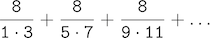
which converges to pi very slowly.
>>> def pi_sum(n):
        total, k = 0, 1
        while k <= n:
            total, k = total + 8 / (k * (k + 2)), k + 4
        return total
>>> pi_sum(100)
3.121594652591009
These three functions clearly share a common underlying pattern. They are for the most part identical, differing only in name, the function of k used to compute the term to be added, and the function that provides the next value of k. We could generate each of the functions by filling in slots in the same template:
def <name>(n):
    total, k = 0, 1
    while k <= n:
        total, k = total + <term>(k), <next>(k)
    return total
The presence of such a common pattern is strong evidence that there is a useful abstraction waiting to be brought to the surface. Each of these functions is a summation of terms. As program designers, we would like our language to be powerful enough so that we can write a function that expresses the concept of summation itself rather than only functions that compute particular sums. We can do so readily in Python by taking the common template shown above and transforming the "slots" into formal parameters:
>>> def summation(n, term, next):
        total, k = 0, 1
        while k <= n:
            total, k = total + term(k), next(k)
        return total
Notice that summation takes as its arguments the upper bound n together with the functions term and next. We can use summation just as we would any function, and it expresses summations succinctly:
>>> def cube(k):
        return pow(k, 3)
>>> def successor(k):
        return k + 1
>>> def sum_cubes(n):
        return summation(n, cube, successor)
>>> sum_cubes(3)
36
Using an identity function that returns its argument, we can also sum integers.
>>> def identity(k):
        return k
>>> def sum_naturals(n):
        return summation(n, identity, successor)
>>> sum_naturals(10)
55
We can also define pi_sum piece by piece, using our summation abstraction to combine components.
>>> def pi_term(k):
        denominator = k * (k + 2)
        return 8 / denominator
>>> def pi_next(k):
        return k + 4
>>> def pi_sum(n):
        return summation(n, pi_term, pi_next)
>>> pi_sum(1e6)
3.1415906535898936
1.6.2 Functions as General Methods
We introduced user-defined functions as a mechanism for abstracting patterns of numerical operations so as to make them independent of the particular numbers involved. With higher-order functions, we begin to see a more powerful kind of abstraction: some functions express general methods of computation, independent of the particular functions they call.
Despite this conceptual extension of what a function means, our environment model of how to evaluate a call expression extends gracefully to the case of higher-order functions, without change. When a user-defined function is applied to some arguments, the formal parameters are bound to the values of those arguments (which may be functions) in a new local frame.
Consider the following example, which implements a general method for iterative improvement and uses it to compute the golden ratio. An iterative improvement algorithm begins with a guess of a solution to an equation. It repeatedly applies an update function to improve that guess, and applies a test to check whether the current guess is "close enough" to be considered correct.
>>> def iter_improve(update, test, guess=1):
        while not test(guess):
            guess = update(guess)
        return guess
The test function typically checks whether two functions, f and g, are near to each other for the value guess. Testing whether f(x) is near to g(x) is again a general method of computation.
>>> def near(x, f, g):
        return approx_eq(f(x), g(x))
A common way to test for approximate equality in programs is to compare the absolute value of the difference between numbers to a small tolerance value.
>>> def approx_eq(x, y, tolerance=1e-5):
        return abs(x - y) < tolerance
The golden ratio, often called phi, is a number that appears frequently in nature, art, and architecture. It can be computed via iter_improve using the golden_update, and it converges when its successor is equal to its square.
>>> def golden_update(guess):
        return 1/guess + 1
>>> def golden_test(guess):
        return near(guess, square, successor)
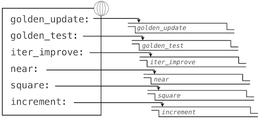
At this point, we have added several bindings to the global frame. The depictions of function values are abbreviated for clarity.
Calling iter_improve with the arguments golden_update and golden_test will compute an approximation to the golden ratio.
>>> iter_improve(golden_update, golden_test)
1.6180371352785146
By tracing through the steps of our evaluation procedure, we can see how this result is computed. First, a local frame for iter_improve is constructed with bindings for update, test, and guess. In the body of iter_improve, the name test is bound to golden_test, which is called on the initial value of guess. In turn, golden_test calls near, creating a third local frame that binds the formal parameters f and g to square and successor.
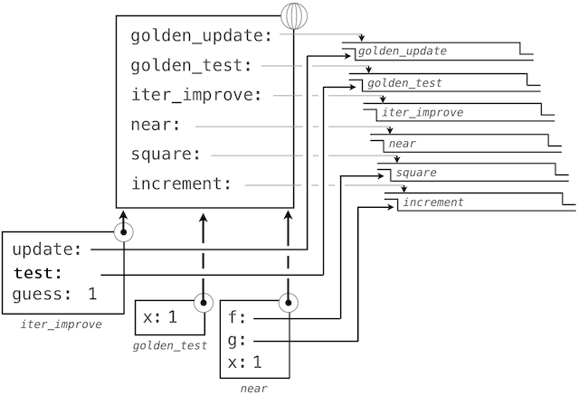
Completing the evaluation of near, we see that the golden_test is False because 1 is not close to 2. Hence, evaluation proceeds with the suite of the while clause, and this mechanical process repeats several times.
This extended example illustrates two related big ideas in computer science. First, naming and functions allow us to abstract away a vast amount of complexity. While each function definition has been trivial, the computational process set in motion by our evaluation procedure appears quite intricate, and we didn't even illustrate the whole thing. Second, it is only by virtue of the fact that we have an extremely general evaluation procedure that small components can be composed into complex processes. Understanding that procedure allows us to validate and inspect the process we have created.
As always, our new general method iter_improve needs a test to check its correctness. The golden ratio can provide such a test, because it also has an exact closed-form solution, which we can compare to this iterative result.
>>> phi = 1/2 + pow(5, 1/2)/2
>>> def near_test():
        assert near(phi, square, successor), 'phi * phi is not near phi + 1'
>>> def iter_improve_test():
        approx_phi = iter_improve(golden_update, golden_test)
        assert approx_eq(phi, approx_phi), 'phi differs from its approximation'
New environment Feature: Higher-order functions.
Extra for experts. We left out a step in the justification of our test. For what range of tolerance values e can you prove that if near(x, square, successor) is true with tolerance value e, then approx_eq(phi, x) is true with the same tolerance?
1.6.3 Defining Functions III: Nested Definitions
The above examples demonstrate how the ability to pass functions as arguments significantly enhances the expressive power of our programming language. Each general concept or equation maps onto its own short function. One negative consequence of this approach to programming is that the global frame becomes cluttered with names of small functions. Another problem is that we are constrained by particular function signatures: the update argument to iter_improve must take exactly one argument. In Python, nested function definitions address both of these problems, but require us to amend our environment model slightly.
Let's consider a new problem: computing the square root of a number. Repeated application of the following update converges to the square root of x:
>>> def average(x, y):
        return (x + y)/2
>>> def sqrt_update(guess, x):
        return average(guess, x/guess)
This two-argument update function is incompatible with iter_improve, and it just provides an intermediate value; we really only care about taking square roots in the end. The solution to both of these issues is to place function definitions inside the body of other definitions.
>>> def square_root(x):
        def update(guess):
            return average(guess, x/guess)
        def test(guess):
            return approx_eq(square(guess), x)
        return iter_improve(update, test)
Like local assignment, local def statements only affect the current local frame. These functions are only in scope while square_root is being evaluated. Consistent with our evaluation procedure, these local def statements don't even get evaluated until square_root is called.
Lexical scope. Locally defined functions also have access to the name bindings in the scope in which they are defined. In this example, update refers to the name x, which is a formal parameter of its enclosing function square_root. This discipline of sharing names among nested definitions is called lexical scoping. Critically, the inner functions have access to the names in the environment where they are defined (not where they are called).
We require two extensions to our environment model to enable lexical scoping.
- Each user-defined function has an associated environment: the environment in which it was defined.
- When a user-defined function is called, its local frame extends the environment associated with the function.
Previous to square_root, all functions were defined in the global environment, and so they were all associated with the global environment. When we evaluate the first two clauses of square_root, we create functions that are associated with a local environment. In the call
>>> square_root(256)
16.00000000000039
the environment first adds a local frame for square_root and evaluates the def statements for update and test (only update is shown).
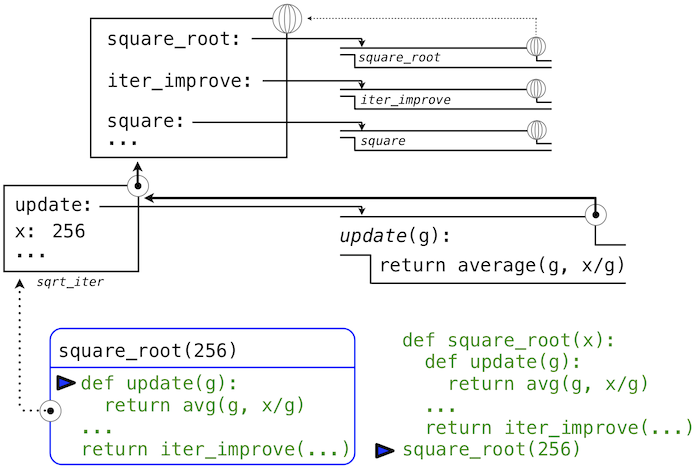
Subsequently, the name update resolves to this newly defined function, which is passed as an argument to iter_improve. Within the body of iter_improve, we must apply our update function to the initial guess of 1. This final application creates an environment for update that begins with a local frame containing only g, but with the preceding frame for square_root still containing a binding for x.
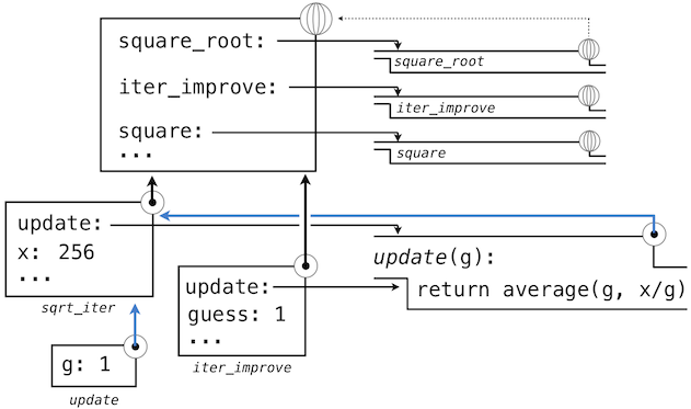
The most crucial part of this evaluation procedure is the transfer of an environment associated with a function to the local frame in which that function is evaluated. This transfer is highlighted by the blue arrows in this diagram.
In this way, the body of update can resolve a value for x. Hence, we realize two key advantages of lexical scoping in Python.
- The names of a local function do not interfere with names external to the function in which it is defined, because the local function name will be bound in the current local environment in which it is defined, rather than the global environment.
- A local function can access the environment of the enclosing function. This is because the body of the local function is evaluated in an environment that extends the evaluation environment in which it is defined.
The update function carries with it some data: the values referenced in the environment in which it was defined. Because they enclose information in this way, locally defined functions are often called closures.
New environment Feature: Local function definition.
1.6.4 Functions as Returned Values
We can achieve even more expressive power in our programs by creating functions whose returned values are themselves functions. An important feature of lexically scoped programming languages is that locally defined functions keep their associated environment when they are returned. The following example illustrates the utility of this feature.
With many simple functions defined, function composition is a natural method of combination to include in our programming language. That is, given two functions f(x) and g(x), we might want to define h(x) = f(g(x)). We can define function composition using our existing tools:
>>> def compose1(f, g):
        def h(x):
            return f(g(x))
        return h
>>> add_one_and_square = compose1(square, successor)
>>> add_one_and_square(12)
169
The 1 in compose1 indicates that the composed functions and returned result all take 1 argument. This naming convention isn't enforced by the interpreter; the 1 is just part of the function name.
At this point, we begin to observe the benefits of our investment in a rich model of computation. No modifications to our environment model are required to support our ability to return functions in this way.
1.6.5 Lambda Expressions
So far, every time we want to define a new function, we need to give it a name. But for other types of expressions, we don’t need to associate intermediate products with a name. That is, we can compute a*b + c*d without having to name the subexpressions a*b or c*d, or the full expression. In Python, we can create function values on the fly using lambda expressions, which evaluate to unnamed functions. A lambda expression evaluates to a function that has a single return expression as its body. Assignment and control statements are not allowed.
Lambda expressions are limited: They are only useful for simple, one-line functions that evaluate and return a single expression. In those special cases where they apply, lambda expressions can be quite expressive.
>>> def compose1(f,g):
        return lambda x: f(g(x))
We can understand the structure of a lambda expression by constructing a corresponding English sentence:
     lambda            x            :          f(g(x))
"A function that    takes x    and returns     f(g(x))"
Some programmers find that using unnamed functions from lambda expressions is shorter and more direct. However, compound lambda expressions are notoriously illegible, despite their brevity. The following definition is correct, but some programmers have trouble understanding it quickly.
>>> compose1 = lambda f,g: lambda x: f(g(x))
In general, Python style prefers explicit def statements to lambda expressions, but allows them in cases where a simple function is needed as an argument or return value.
Such stylistic rules are merely guidelines; you can program any way you wish. However, as you write programs, think about the audience of people who might read your program one day. If you can make your program easier to interpret, you will do those people a favor.
The term lambda is a historical accident resulting from the incompatibility of written mathematical notation and the constraints of early type-setting systems.
It may seem perverse to use lambda to introduce a procedure/function. The notation goes back to Alonzo Church, who in the 1930's started with a "hat" symbol; he wrote the square function as "ŷ . y × y". But frustrated typographers moved the hat to the left of the parameter and changed it to a capital lambda: "Λy . y × y"; from there the capital lambda was changed to lowercase, and now we see "λy . y × y" in math books and (lambda (y) (* y y)) in Lisp.
—Peter Norvig (norvig.com/lispy2.html)
Despite their unusual etymology, lambda expressions and the corresponding formal language for function application, the lambda calculus, are fundamental computer science concepts shared far beyond the Python programming community. We will revisit this topic when we study the design of interpreters in Chapter 3.
1.6.6 Example: Newton's Method
This final extended example shows how function values, local defintions, and lambda expressions can work together to express general ideas concisely.
Newton's method is a classic iterative approach to finding the arguments of a mathematical function that yield a return value of 0. These values are called roots of a single-argument mathematical function. Finding a root of a function is often equivalent to solving a related math problem.
- The square root of 16 is the value x such that: square(x) - 16 = 0
- The log base 2 of 32 (i.e., the exponent to which we would raise 2 to get 32) is the value x such that: pow(2, x) - 32 = 0
Thus, a general method for finding roots will also provide us an algorithm to compute square roots and logarithms. Moreover, the equations for which we want to compute roots only contain simpler operations: multiplication and exponentiation.
A comment before we proceed: it is easy to take for granted the fact that we know how to compute square roots and logarithms. Not just Python, but your phone, your pocket calculator, and perhaps even your watch can do so for you. However, part of learning computer science is understanding how quantities like these can be computed, and the general approach presented here is applicable to solving a large class of equations beyond those built into Python.
Before even beginning to understand Newton's method, we can start programming; this is the power of functional abstractions. We simply translate our previous statements into code.
>>> def square_root(a):
        return find_root(lambda x: square(x) - a)
>>> def logarithm(a, base=2):
        return find_root(lambda x: pow(base, x) - a)
Of course, we cannot apply any of these functions until we define find_root, and so we need to understand how Newton's method works.
Newton's method is also an iterative improvement algorithm: it improves a guess of the root for any function that is differentiable. Notice that both of our functions of interest change smoothly; graphing x versus f(x) for
- f(x) = square(x) - 16 (light curve)
- f(x) = pow(2, x) - 32 (dark curve)
on a 2-dimensional plane shows that both functions produce a smooth curve without kinks that crosses 0 at the appropriate point.
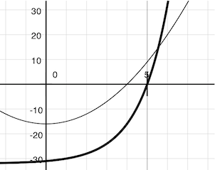
Because they are smooth (differentiable), these curves can be approximated by a line at any point. Newton's method follows these linear approximations to find function roots.
Imagine a line through the point (x, f(x)) that has the same slope as the curve for function f(x) at that point. Such a line is called the tangent, and its slope is called the derivative of f at x.
This line's slope is the ratio of the change in function value to the change in function argument. Hence, translating x by f(x) divided by the slope will give the argument value at which this tangent line touches 0.
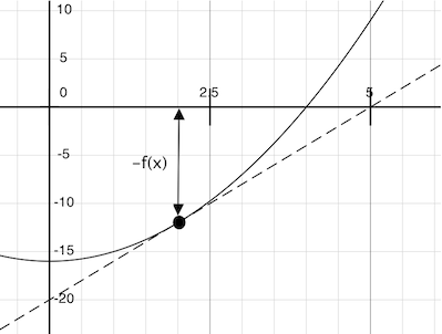
Our Newton update expresses the computational process of following this tangent line to 0. We approximate the derivative of the function by computing its slope over a very small interval.
>>> def approx_derivative(f, x, delta=1e-5):
        df = f(x + delta) - f(x)
        return df/delta
>>> def newton_update(f):
        def update(x):
            return x - f(x) / approx_derivative(f, x)
        return update
Finally, we can define the find_root function in terms of newton_update, our iterative improvement algorithm, and a test to see if f(x) is near 0. We supply a larger initial guess to improve performance for logarithm.
>>> def find_root(f, initial_guess=10):
        def test(x):
            return approx_eq(f(x), 0)
        return iter_improve(newton_update(f), test, initial_guess)
>>> square_root(16)
4.000000000026422
>>> logarithm(32, 2)
5.000000094858201
As you experiment with Newton's method, be aware that it will not always converge. The initial guess of iter_improve must be sufficiently close to the root, and various conditions about the function must be met. Despite this shortcoming, Newton's method is a powerful general computational method for solving differentiable equations. In fact, very fast algorithms for logarithms and large integer division employ variants of the technique.
1.6.7 Abstractions and First-Class Functions
We began this section with the observation that user-defined functions are a crucial abstraction mechanism, because they permit us to express general methods of computing as explicit elements in our programming language. Now we've seen how higher-order functions permit us to manipulate these general methods to create further abstractions.
As programmers, we should be alert to opportunities to identify the underlying abstractions in our programs, to build upon them, and generalize them to create more powerful abstractions. This is not to say that one should always write programs in the most abstract way possible; expert programmers know how to choose the level of abstraction appropriate to their task. But it is important to be able to think in terms of these abstractions, so that we can be ready to apply them in new contexts. The significance of higher-order functions is that they enable us to represent these abstractions explicitly as elements in our programming language, so that they can be handled just like other computational elements.
In general, programming languages impose restrictions on the ways in which computational elements can be manipulated. Elements with the fewest restrictions are said to have first-class status. Some of the "rights and privileges" of first-class elements are:
- They may be bound to names.
- They may be passed as arguments to functions.
- They may be returned as the results of functions.
- They may be included in data structures.
Python awards functions full first-class status, and the resulting gain in expressive power is enormous. Control structures, on the other hand, do not: you cannot pass if to a function the way you can sum.
1.6.8 Function Decorators
Python provides special syntax to apply higher-order functions as part of executing a def statement, called a decorator. Perhaps the most common example is a trace.
>>> def trace1(fn):
        def wrapped(x):
            print('-> ', fn, '(', x, ')')
            return fn(x)
        return wrapped
>>> @trace1
    def triple(x):
        return 3 * x
>>> triple(12)
->  <function triple at 0x102a39848> ( 12 )
36
In this example, A higher-order function trace1 is defined, which returns a function that precedes a call to its argument with a print statement that outputs the argument. The def statement for triple has an annototation, @trace1, which affects the execution rule for def. As usual, the function triple is created. However, the name triple is not bound to this function. Instead, the name triple is bound to the returned function value of calling trace1 on the newly defined triple function. In code, this decorator is equivalent to:
>>> def triple(x):
        return 3 * x
>>> triple = trace1(triple)
In the projects for this course, decorators are used for tracing, as well as selecting which functions to call when a program is run from the command line.
Extra for experts. The actual rule is that the decorator symbol @ may be followed by an expression (@trace1 is just a simple expression consisting of a single name). Any expression producing a suitable value is allowed. For example, with a suitable definition, you could define a decorator check_range so that decorating a function definition with @check_range(1, 10) would cause the function's results to be checked to make sure they are integers between 1 and 10. The call check_range(1,10) would return a function that would then be applied to the newly defined function before it is bound to the name in the def statement. A short tutorial on decorators by Ariel Ortiz gives further examples for interested students.