3.1.1   Programming Languages

In fact, we can regard many programs as interpreters for some language. For example, the constraint propagator from the previous chapter has its own primitives and means of combination. The constraint language was quite specialized: it provided a declarative method for describing a certain class of mathematical relations, not a fully general language for describing computation. While we have been designing languages of a sort already, the material of this chapter will greatly expand the range of languages we can interpret.

Programming languages vary widely in their syntactic structures, features, and domain of application. Among general purpose programming languages, the constructs of function definition and function application are pervasive. On the other hand, powerful languages exist that do not include an object system, higher-order functions, or even control constructs like while and for statements. To illustrate just how different languages can be, we will introduce Logo as an example of a powerful and expressive programming language that includes very few advanced features.

In this chapter, we study the design of interpreters and the computational processes that they create when executing programs. The prospect of designing an interpreter for a general programming language may seem daunting. After all, interpreters are programs that can carry out any possible computation, depending on their input. However, typical interpreters have an elegant common structure: two mutually recursive functions. The first evaluates expressions in environments; the second applies functions to arguments.

These functions are recursive in that they are defined in terms of each other: applying a function requires evaluating the expressions in its body, while evaluating an expression may involve applying one or more functions. The next two sections of this chapter focus on recursive functions and data structures, which will prove essential to understanding the design of an interpreter. The end of the chapter focuses on two new languages and the task of implementing interpreters for them.

3.2.1   Recursive Functions

A function is called recursive if the body of that function calls the function itself, either directly or indirectly. That is, the process of executing the body of a recursive function may in turn require applying that function again. Recursive functions do not require any special syntax in Python, but they do require some care to define correctly.

As an introduction to recursive functions, we begin with the task of converting an English word into its Pig Latin equivalent. Pig Latin is a secret language: one that applies a simple, deterministic transformation to each word that veils the meaning of the word. Thomas Jefferson was supposedly an early adopter. The Pig Latin equivalent of an English word moves the initial consonant cluster (which may be empty) from the beginning of the word to the end and follows it by the "-ay" vowel. Hence, the word "pun" becomes "unpay", "stout" becomes "outstay", and "all" becomes "allay".

>>> def pig_latin(w):
        """Return the Pig Latin equivalent of English word w."""
        if starts_with_a_vowel(w):
            return w + 'ay'
        return pig_latin(w[1:] + w[0])

>>> def starts_with_a_vowel(w):
        """Return whether w begins with a vowel."""
        return w[0].lower() in 'aeiou'

The idea behind this definition is that the Pig Latin variant of a string that starts with a consonant is the same as the Pig Latin variant of another string: that which is created by moving the first letter to the end. Hence, the Pig Latin word for "sending" is the same as for "endings" (endingsay), and the Pig Latin word for "smother" is the same as the Pig Latin word for "mothers" (othersmay). Moreover, moving one consonant from the beginning of the word to the end results in a simpler problem with fewer initial consonants. In the case of "sending", moving the "s" to the end gives a word that starts with a vowel, and so our work is done.

This definition of pig_latin is both complete and correct, even though the pig_latin function is called within its own body.

>>> pig_latin('pun')
'unpay'

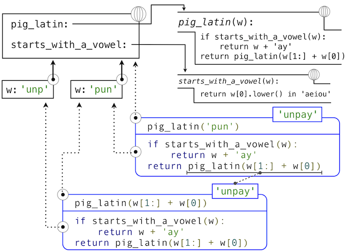
The idea of being able to define a function in terms of itself may be disturbing; it may seem unclear how such a "circular" definition could make sense at all, much less specify a well-defined process to be carried out by a computer. We can, however, understand precisely how this recursive function applies successfully using our environment model of computation. The environment diagram and expression tree that depict the evaluation of pig_latin('pun') appear below.

The steps of the Python evaluation procedures that produce this result are:

1. The def statement for pig_latin is executed, which

1. Creates a new pig_latin function object with the stated body, and
2. Binds the name pig_latin to that function in the current (global) frame

2. The def statement for starts_with_a_vowel is executed similarly
3. The call expression pig_latin('pun') is evaluated by

1. Evaluating the operator and operand sub-expressions by

1. Looking up the name pig_latin that is bound to the pig_latin function
2. Evaluating the operand string literal to the string object 'pun'

2. Applying the function pig_latin to the argument 'pun' by

1. Adding a local frame that extends the global frame
2. Binding the formal parameter w to the argument 'pun' in that frame
3. Executing the body of pig_latin in the environment that starts with that frame:

1. The initial conditional statement has no effect, because the header expression evaluates to False.
2. The final return expression pig_latin(w[1:] + w[0]) is evaluated by

1. Looking up the name pig_latin that is bound to the pig_latin function
2. Evaluating the operand expression to the string object 'unp'
3. Applying pig_latin to the argument 'unp', which returns the desired result from the suite of the conditional statement in the body of pig_latin.

As this example illustrates, a recursive function applies correctly, despite its circular character. The pig_latin function is applied twice, but with a different argument each time. Although the second call comes from the body of pig_latin itself, looking up that function by name succeeds because the name pig_latin is bound in the environment before its body is executed.

This example also illustrates how Python's recursive evaluation procedure can interact with a recursive function to evolve a complex computational process with many nested steps, even though the function definition may itself contain very few lines of code.

3.2.2   The Anatomy of Recursive Functions

A common pattern can be found in the body of many recursive functions. The body begins with a base case, a conditional statement that defines the behavior of the function for the inputs that are simplest to process. In the case of pig_latin, the base case occurs for any argument that starts with a vowel. In this case, there is no work left to be done but return the argument with "ay" added to the end. Some recursive functions will have multiple base cases.

The base cases are then followed by one or more recursive calls. Recursive calls require a certain character: they must simplify the original problem. In the case of pig_latin, the more initial consonants in w, the more work there is left to do. In the recursive call, pig_latin(w[1:] + w[0]), we call pig_latin on a word that has one fewer initial consonant -- a simpler problem. Each successive call to pig_latin will be simpler still until the base case is reached: a word with no initial consonants.

Recursive functions express computation by simplifying problems incrementally. They often operate on problems in a different way than the iterative approaches that we have used in the past. Consider a function fact to compute n factorial, where for example fact(4) computes \(4! = 4 \cdot 3 \cdot 2 \cdot 1 = 24\).

A natural implementation using a while statement accumulates the total by multiplying together each positive integer up to n.

>>> def fact_iter(n):
        total, k = 1, 1
        while k <= n:
            total, k = total * k, k + 1
        return total

>>> fact_iter(4)
24

On the other hand, a recursive implementation of factorial can express fact(n) in terms of fact(n-1), a simpler problem. The base case of the recursion is the simplest form of the problem: fact(1) is 1.

>>> def fact(n):
        if n == 1:
            return 1
        return n * fact(n-1)

>>> fact(4)
24

The correctness of this function is easy to verify from the standard definition of the mathematical function for factorial:

\[\begin{array}{l l} (n-1)! &= (n-1) \cdot (n-2) \cdot \dots \cdot 1 \\ n! &= n \cdot (n-1) \cdot (n-2) \cdot \dots \cdot 1 \\ n! &= n \cdot (n-1)! \end{array}\]

These two factorial functions differ conceptually. The iterative function constructs the result from the base case of 1 to the final total by successively multiplying in each term. The recursive function, on the other hand, constructs the result directly from the final term, n, and the result of the simpler problem, fact(n-1).

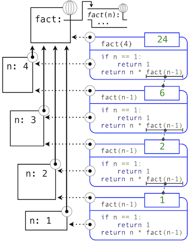
As the recursion "unwinds" through successive applications of the fact function to simpler and simpler problem instances, the result is eventually built starting from the base case. The diagram below shows how the recursion ends by passing the argument 1 to fact, and how the result of each call depends on the next until the base case is reached.

While we can unwind the recursion using our model of computation, it is often clearer to think about recursive calls as functional abstractions. That is, we should not care about how fact(n-1) is implemented in the body of fact; we should simply trust that it computes the factorial of n-1. Treating a recursive call as a functional abstraction has been called a recursive leap of faith. We define a function in terms of itself, but simply trust that the simpler cases will work correctly when verifying the correctness of the function. In this example, we trust that fact(n-1) will correctly compute (n-1)!; we must only check that n! is computed correctly if this assumption holds. In this way, verifying the correctness of a recursive function is a form of proof by induction.

The functions fact_iter and fact also differ because the former must introduce two additional names, total and k, that are not required in the recursive implementation. In general, iterative functions must maintain some local state that changes throughout the course of computation. At any point in the iteration, that state characterizes the result of completed work and the amount of work remaining. For example, when k is 3 and total is 2, there are still two terms remaining to be processed, 3 and 4. On the other hand, fact is characterized by its single argument n. The state of the computation is entirely contained within the structure of the expression tree, which has return values that take the role of total, and binds n to different values in different frames rather than explicitly tracking k.

Recursive functions can rely more heavily on the interpreter itself, by storing the state of the computation as part of the expression tree and environment, rather than explicitly using names in the local frame. For this reason, recursive functions are often easier to define, because we do not need to try to determine the local state that must be maintained across iterations. On the other hand, learning to recognize the computational processes evolved by recursive functions can require some practice.

3.2.3   Tree Recursion

Another common pattern of computation is called tree recursion. As an example, consider computing the sequence of Fibonacci numbers, in which each number is the sum of the preceding two.

>>> def fib(n):
        if n == 1:
            return 0
        if n == 2:
            return 1
        return fib(n-2) + fib(n-1)

>>> fib(6)
5

This recursive definition is tremendously appealing relative to our previous attempts: it exactly mirrors the familiar definition of Fibonacci numbers. Consider the pattern of computation that results from evaluating fib(6), shown below. To compute fib(6), we compute fib(5) and fib(4). To compute fib(5), we compute fib(4) and fib(3). In general, the evolved process looks like a tree (the diagram below is not a full expression tree, but instead a simplified depiction of the process; a full expression tree would have the same general structure). Each blue dot indicates a completed computation of a Fibonacci number in the traversal of this tree.

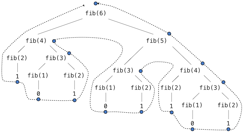
Functions that call themselves multiple times in this way are said to be tree recursive. This function is instructive as a prototypical tree recursion, but it is a terrible way to compute Fibonacci numbers because it does so much redundant computation. Notice that the entire computation of fib(4) -- almost half the work -- is duplicated. In fact, it is not hard to show that the number of times the function will compute fib(1) or fib(2) (the number of leaves in the tree, in general) is precisely fib(n+1). To get an idea of how bad this is, one can show that the value of fib(n) grows exponentially with n. Thus, the process uses a number of steps that grows exponentially with the input.

We have already seen an iterative implementation of Fibonacci numbers, repeated here for convenience.

>>> def fib_iter(n):
        prev, curr = 1, 0  # curr is the first Fibonacci number.
        for _ in range(n-1):
             prev, curr = curr, prev + curr
        return curr

The state that we must maintain in this case consists of the current and previous Fibonacci numbers. Implicitly the for statement also keeps track of the iteration count. This definition does not reflect the standard mathematical definition of Fibonacci numbers as clearly as the recursive approach. However, the amount of computation required in the iterative implementation is only linear in n, rather than exponential. Even for small values of n, this difference can be enormous.

One should not conclude from this difference that tree-recursive processes are useless. When we consider processes that operate on hierarchically structured data rather than numbers, we will find that tree recursion is a natural and powerful tool. Furthermore, tree-recursive processes can often be made more efficient.

Memoization. A powerful technique for increasing the efficiency of recursive functions that repeat computation is called memoization. A memoized function will store the return value for any arguments it has previously received. A second call to fib(4) would not evolve the same complex process as the first, but instead would immediately return the stored result computed by the first call.

Memoization can be expressed naturally as a higher-order function, which can also be used as a decorator. The definition below creates a cache of previously computed results, indexed by the arguments from which they were computed. The use of a dictionary will require that the argument to the memoized function be immutable in this implementation.

>>> def memo(f):
        """Return a memoized version of single-argument function f."""
        cache = {}
        def memoized(n):
            if n not in cache:
                cache[n] = f(n)
            return cache[n]
        return memoized

>>> fib = memo(fib)
>>> fib(40)
63245986

The amount of computation time saved by memoization in this case is substantial. The memoized, recursive fib function and the iterative fib_iter function both require an amount of time to compute that is only a linear function of their input n. To compute fib(40), the body of fib is executed 40 times, rather than 102,334,155 times in the unmemoized recursive case.

Space. To understand the space requirements of a function, we must specify generally how memory is used, preserved, and reclaimed in our environment model of computation. In evaluating an expression, we must preserve all active environments and all values and frames referenced by those environments. An environment is active if it provides the evaluation context for some expression in the current branch of the expression tree.

For example, when evaluating fib, the interpreter proceeds to compute each value in the order shown previously, traversing the structure of the tree. To do so, it only needs to keep track of those nodes that are above the current node in the tree at any point in the computation. The memory used to evaluate the rest of the branches can be reclaimed because it cannot affect future computation. In general, the space required for tree-recursive functions will be proportional to the maximum depth of the tree.

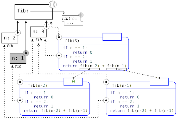
The diagram below depicts the environment and expression tree generated by evaluating fib(3). In the process of evaluating the return expression for the initial application of fib, the expression fib(n-2) is evaluated, yielding a value of 0. Once this value is computed, the corresponding environment frame (grayed out) is no longer needed: it is not part of an active environment. Thus, a well-designed interpreter can reclaim the memory that was used to store this frame. On the other hand, if the interpreter is currently evaluating fib(n-1), then the environment created by this application of fib (in which n is 2) is active. In turn, the environment originally created to apply fib to 3 is active because its value has not yet been successfully computed.

In the case of memo, the environment associated with the function it returns (which contains cache) must be preserved as long as some name is bound to that function in an active environment. The number of entries in the cache dictionary grows linearly with the number of unique arguments passed to fib, which scales linearly with the input. On the other hand, the iterative implementation requires only two numbers to be tracked during computation: prev and curr, giving it a constant size.

Memoization exemplifies a common pattern in programming that computation time can often be decreased at the expense of increased use of space, or vis versa.

3.2.4   Example: Counting Change

Consider the following problem: How many different ways can we make change of $1.00, given half-dollars, quarters, dimes, nickels, and pennies? More generally, can we write a function to compute the number of ways to change any given amount of money using any set of currency denominations?

This problem has a simple solution as a recursive function. Suppose we think of the types of coins available as arranged in some order, say from most to least valuable.

The number of ways to change an amount a using n kinds of coins equals

1. the number of ways to change a using all but the first kind of coin, plus
2. the number of ways to change the smaller amount a - d using all n kinds of coins, where d is the denomination of the first kind of coin.

To see why this is true, observe that the ways to make change can be divided into two groups: those that do not use any of the first kind of coin, and those that do. Therefore, the total number of ways to make change for some amount is equal to the number of ways to make change for the amount without using any of the first kind of coin, plus the number of ways to make change assuming that we do use the first kind of coin at least once. But the latter number is equal to the number of ways to make change for the amount that remains after using a coin of the first kind.

Thus, we can recursively reduce the problem of changing a given amount to the problem of changing smaller amounts using fewer kinds of coins. Consider this reduction rule carefully and convince yourself that we can use it to describe an algorithm if we specify the following base cases:

1. If a is exactly 0, we should count that as 1 way to make change.
2. If a is less than 0, we should count that as 0 ways to make change.
3. If n is 0, we should count that as 0 ways to make change.

We can easily translate this description into a recursive function:

>>> def count_change(a, kinds=(50, 25, 10, 5, 1)):
        """Return the number of ways to change amount a using coin kinds."""
        if a == 0:
            return 1
        if a < 0 or len(kinds) == 0:
            return 0
        d = kinds[0]
        return count_change(a, kinds[1:]) + count_change(a - d, kinds)

>>> count_change(100)
292

The count_change function generates a tree-recursive process with redundancies similar to those in our first implementation of fib. It will take quite a while for that 292 to be computed, unless we memoize the function. On the other hand, it is not obvious how to design an iterative algorithm for computing the result, and we leave this problem as a challenge.

3.2.5   Orders of Growth

The previous examples illustrate that processes can differ considerably in the rates at which they consume the computational resources of space and time. One convenient way to describe this difference is to use the notion of order of growth to obtain a coarse measure of the resources required by a process as the inputs become larger.

Let \(n\) be a parameter that measures the size of the problem, and let \(R(n)\) be the amount of resources the process requires for a problem of size \(n\). In our previous examples we took \(n\) to be the number for which a given function is to be computed, but there are other possibilities. For instance, if our goal is to compute an approximation to the square root of a number, we might take \(n\) to be the number of digits of accuracy required. In general there are a number of properties of the problem with respect to which it will be desirable to analyze a given process. Similarly, \(R(n)\) might measure the amount of memory used, the number of elementary machine operations performed, and so on. In computers that do only a fixed number of operations at a time, the time required to evaluate an expression will be proportional to the number of elementary machine operations performed in the process of evaluation.

We say that \(R(n)\) has order of growth \(\Theta(f(n))\), written \(R(n) = \Theta(f(n))\) (pronounced "theta of \(f(n)\)"), if there are positive constants \(k_1\) and \(k_2\) independent of \(n\) such that

\[k_1 \cdot f(n) \leq R(n) \leq k_2 \cdot f(n)\]

for any sufficiently large value of \(n\). In other words, for large \(n\), the value \(R(n)\) is sandwiched between two values that both scale with \(f(n)\):

• A lower bound \(k_1 \cdot f(n)\) and
• An upper bound \(k_2 \cdot f(n)\)

For instance, the number of steps to compute \(n!\) grows proportionally to the input \(n\). Thus, the steps required for this process grows as \(\Theta(n)\). We also saw that the space required for the recursive implementation fact grows as \(\Theta(n)\). By contrast, the iterative implementation fact_iter takes a similar number of steps, but the space it requires stays constant. In this case, we say that the space grows as \(\Theta(1)\).

The number of steps in our tree-recursive Fibonacci computation fib grows exponentially in its input \(n\). In particular, one can show that the nth Fibonacci number is the closest integer to

\[\frac{\phi^{n-2}}{\sqrt{5}}\]

where \(\phi\) is the golden ratio:

\[\phi = \frac{1 + \sqrt{5}}{2} \approx 1.6180\]

We also stated that the number of steps scales with the resulting value, and so the tree-recursive process requires \(\Theta(\phi^n)\) steps, a function that grows exponentially with \(n\).

Orders of growth provide only a crude description of the behavior of a process. For example, a process requiring \(n^2\) steps and a process requiring \(1000 \cdot n^2\) steps and a process requiring \(3 \cdot n^2 + 10 \cdot n + 17\) steps all have \(\Theta(n^2)\) order of growth. There are certainly cases in which an order of growth analysis is too coarse a method for deciding between two possible implementations of a function.

However, order of growth provides a useful indication of how we may expect the behavior of the process to change as we change the size of the problem. For a \(\Theta(n)\) (linear) process, doubling the size will roughly double the amount of resources used. For an exponential process, each increment in problem size will multiply the resource utilization by a constant factor. The next example examines an algorithm whose order of growth is logarithmic, so that doubling the problem size increases the resource requirement by only a constant amount.

3.2.6   Example: Exponentiation

Consider the problem of computing the exponential of a given number. We would like a function that takes as arguments a base b and a positive integer exponent n and computes \(b^n\). One way to do this is via the recursive definition

\[\begin{array}{l l} b^n &= b \cdot b^{n-1} \\ b^0 &= 1 \end{array}\]

which translates readily into the recursive function

>>> def exp(b, n):
        if n == 0:
            return 1
        return b * exp(b, n-1)

This is a linear recursive process that requires \(\Theta(n)\) steps and \(\Theta(n)\) space. Just as with factorial, we can readily formulate an equivalent linear iteration that requires a similar number of steps but constant space.

>>> def exp_iter(b, n):
        result = 1
        for _ in range(n):
            result = result * b
        return result

We can compute exponentials in fewer steps by using successive squaring. For instance, rather than computing \(b^8\) as

\[b \cdot (b \cdot (b \cdot (b \cdot (b \cdot (b \cdot (b \cdot b))))))\]

we can compute it using three multiplications:

\[\begin{array}{l l} b^2 &= b \cdot b \\ b^4 &= b^2 \cdot b^2 \\ b^8 &= b^4 \cdot b^4 \end{array}\]

This method works fine for exponents that are powers of 2. We can also take advantage of successive squaring in computing exponentials in general if we use the recursive rule

\[b^n = \left\{\begin{array}{l l} (b^{\frac{1}{2} n})^2 & \mbox{if $n$ is even} \\ b \cdot b^{n-1} & \mbox{if $n$ is odd} \end{array} \right.\]

We can express this method as a recursive function as well:

>>> def square(x):
        return x*x

>>> def fast_exp(b, n):
        if n == 0:
            return 1
        if n % 2 == 0:
            return square(fast_exp(b, n//2))
        else:
            return b * fast_exp(b, n-1)

>>> fast_exp(2, 100)
1267650600228229401496703205376

The process evolved by fast_exp grows logarithmically with n in both space and number of steps. To see this, observe that computing \(b^{2n}\) using fast_exp requires only one more multiplication than computing \(b^n\). The size of the exponent we can compute therefore doubles (approximately) with every new multiplication we are allowed. Thus, the number of multiplications required for an exponent of n grows about as fast as the logarithm of n base 2. The process has \(\Theta(\log n)\) growth. The difference between \(\Theta(\log n)\) growth and \(\Theta(n)\) growth becomes striking as \(n\) becomes large. For example, fast_exp for n of 1000 requires only 14 multiplications instead of 1000.

3.3.1   Processing Recursive Lists

Recall that the recursive list abstract data type represented a list as a first element and the rest of the list. We previously implemented recursive lists using functions, but at this point we can re-implement them using a class. Below, the length (__len__) and element selection (__getitem__) functions are written recursively to demonstrate typical patterns for processing recursive lists.

>>> class Rlist(object):
        """A recursive list consisting of a first element and the rest."""
        class EmptyList(object):
            def __len__(self):
                return 0
        empty = EmptyList()
        def __init__(self, first, rest=empty):
            self.first = first
            self.rest = rest
        def __repr__(self):
            args = repr(self.first)
            if self.rest is not Rlist.empty:
                args += ', {0}'.format(repr(self.rest))
            return 'Rlist({0})'.format(args)
        def __len__(self):
            return 1 + len(self.rest)
        def __getitem__(self, i):
            if i == 0:
                return self.first
            return self.rest[i-1]

The definitions of __len__ and __getitem__ are in fact recursive, although not explicitly so. The built-in Python function len looks for a method called __len__ when applied to a user-defined object argument. Likewise, the subscript operator looks for a method called __getitem__. Thus, these definitions will end up calling themselves. Recursive calls on the rest of the list are a ubiquitous pattern in recursive list processing. This class definition of a recursive list interacts properly with Python's built-in sequence and printing operations.

>>> s = Rlist(1, Rlist(2, Rlist(3)))
>>> s.rest
Rlist(2, Rlist(3))
>>> len(s)
3
>>> s[1]
2

Operations that create new lists are particularly straightforward to express using recursion. For example, we can define a function extend_rlist, which takes two recursive lists as arguments and combines the elements of both into a new list.

>>> def extend_rlist(s1, s2):
        if s1 is Rlist.empty:
            return s2
        return Rlist(s1.first, extend_rlist(s1.rest, s2))

>>> extend_rlist(s.rest, s)
Rlist(2, Rlist(3, Rlist(1, Rlist(2, Rlist(3)))))

Likewise, mapping a function over a recursive list exhibits a similar pattern.

>>> def map_rlist(s, fn):
        if s is Rlist.empty:
            return s
        return Rlist(fn(s.first), map_rlist(s.rest, fn))

>>> map_rlist(s, square)
Rlist(1, Rlist(4, Rlist(9)))

Filtering includes an additional conditional statement, but otherwise has a similar recursive structure.

>>> def filter_rlist(s, fn):
        if s is Rlist.empty:
            return s
        rest = filter_rlist(s.rest, fn)
        if fn(s.first):
            return Rlist(s.first, rest)
        return rest

>>> filter_rlist(s, lambda x: x % 2 == 1)
Rlist(1, Rlist(3))

Recursive implementations of list operations do not, in general, require local assignment or while statements. Instead, recursive lists are taken apart and constructed incrementally as a consequence of function application. As a result, they have linear orders of growth in both the number of steps and space required.

3.3.2   Hierarchical Structures

Hierarchical structures result from the closure property of data, which asserts for example that tuples can contain other tuples. For instance, consider this nested representation of the numbers 1 through 4.

>>> ((1, 2), 3, 4)
((1, 2), 3, 4)

This tuple is a length-three sequence, of which the first element is itself a tuple. A box-and-pointer diagram of this nested structure shows that it can also be thought of as a tree with four leaves, each of which is a number.

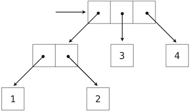
In a tree, each subtree is itself a tree. As a base condition, any bare element that is not a tuple is itself a simple tree, one with no branches. That is, the numbers are all trees, as is the pair (1, 2) and the structure as a whole.

Recursion is a natural tool for dealing with tree structures, since we can often reduce operations on trees to operations on their branches, which reduce in turn to operations on the branches of the branches, and so on, until we reach the leaves of the tree. As an example, we can implement a count_leaves function, which returns the total number of leaves of a tree.

>>> def count_leaves(tree):
        if type(tree) != tuple:
            return 1
        return sum(map(count_leaves, tree))

>>> t = ((1, 2), 3, 4)
>>> count_leaves(t)
4
>>> big_tree = ((t, t), 5)
>>> big_tree
((((1, 2), 3, 4), ((1, 2), 3, 4)), 5)
>>> count_leaves(big_tree)
9

Just as map is a powerful tool for dealing with sequences, mapping and recursion together provide a powerful general form of computation for manipulating trees. For instance, we can square all leaves of a tree using a higher-order recursive function map_tree that is structured quite similarly to count_leaves.

>>> def map_tree(tree, fn):
        if type(tree) != tuple:
            return fn(tree)
        return tuple(map_tree(branch, fn) for branch in tree)

>>> map_tree(big_tree, square)
((((1, 4), 9, 16), ((1, 4), 9, 16)), 25)

Internal values. The trees described above have values only at the leaves. Another common representation of tree-structured data has values for the internal nodes of the tree as well. We can represent such trees using a class.

>>> class Tree(object):
        def __init__(self, entry, left=None, right=None):
            self.entry = entry
            self.left = left
            self.right = right
        def __repr__(self):
            args = repr(self.entry)
            if self.left or self.right:
                args += ', {0}, {1}'.format(repr(self.left), repr(self.right))
            return 'Tree({0})'.format(args)

The Tree class can represent, for instance, the values computed in an expression tree for the recursive implementation of fib, the function for computing Fibonacci numbers. The function fib_tree(n) below returns a Tree that has the nth Fibonacci number as its entry and a trace of all previously computed Fibonacci numbers within its branches.

>>> def fib_tree(n):
        """Return a Tree that represents a recursive Fibonacci calculation."""
        if n == 1:
            return Tree(0)
        if n == 2:
            return Tree(1)
        left = fib_tree(n-2)
        right = fib_tree(n-1)
        return Tree(left.entry + right.entry, left, right)

>>> fib_tree(5)
Tree(3, Tree(1, Tree(0), Tree(1)), Tree(2, Tree(1), Tree(1, Tree(0), Tree(1))))

This example shows that expression trees can be represented programmatically using tree-structured data. This connection between nested expressions and tree-structured data type plays a central role in our discussion of designing interpreters later in this chapter.

3.3.3   Sets

In addition to the list, tuple, and dictionary, Python has a fourth built-in container type called a set. Set literals follow the mathematical notation of elements enclosed in braces. Duplicate elements are removed upon construction. Sets are unordered collections, and so the printed ordering may differ from the element ordering in the set literal.

>>> s = {3, 2, 1, 4, 4}
>>> s
{1, 2, 3, 4}

Python sets support a variety of operations, including membership tests, length computation, and the standard set operations of union and intersection

>>> 3 in s
True
>>> len(s)
4
>>> s.union({1, 5})
{1, 2, 3, 4, 5}
>>> s.intersection({6, 5, 4, 3})
{3, 4}

In addition to union and intersection, Python sets support several other methods. The predicates isdisjoint, issubset, and issuperset provide set comparison. Sets are mutable, and can be changed one element at a time using add, remove, discard, and pop. Additional methods provide multi-element mutations, such as clear and update. The Python documentation for sets should be sufficiently intelligible at this point of the course to fill in the details.

Implementing sets. Abstractly, a set is a collection of distinct objects that supports membership testing, union, intersection, and adjunction. Adjoining an element and a set returns a new set that contains all of the original set's elements along with the new element, if it is distinct. Union and intersection return the set of elements that appear in either or both sets, respectively. As with any data abstraction, we are free to implement any functions over any representation of sets that provides this collection of behaviors.

In the remainder of this section, we consider three different methods of implementing sets that vary in their representation. We will characterize the efficiency of these different representations by analyzing the order of growth of set operations. We will use our Rlist and Tree classes from earlier in this section, which allow for simple and elegant recursive solutions for elementary set operations.

Sets as unordered sequences. One way to represent a set is as a sequence in which no element appears more than once. The empty set is represented by the empty sequence. Membership testing walks recursively through the list.

>>> def empty(s):
        return s is Rlist.empty

>>> def set_contains(s, v):
        """Return True if and only if set s contains v."""
        if empty(s):
            return False
        elif s.first == v:
            return True
        return set_contains(s.rest, v)

>>> s = Rlist(1, Rlist(2, Rlist(3)))
>>> set_contains(s, 2)
True
>>> set_contains(s, 5)
False

This implementation of set_contains requires \(\Theta(n)\) time to test membership of an element, where \(n\) is the size of the set s. Using this linear-time function for membership, we can adjoin an element to a set, also in linear time.

>>> def adjoin_set(s, v):
        """Return a set containing all elements of s and element v."""
        if set_contains(s, v):
            return s
        return Rlist(v, s)

>>> t = adjoin_set(s, 4)
>>> t
Rlist(4, Rlist(1, Rlist(2, Rlist(3))))

In designing a representation, one of the issues with which we should be concerned is efficiency. Intersecting two sets set1 and set2 also requires membership testing, but this time each element of set1 must be tested for membership in set2, leading to a quadratic order of growth in the number of steps, \(\Theta(n^2)\), for two sets of size \(n\).

>>> def intersect_set(set1, set2):
        """Return a set containing all elements common to set1 and set2."""
        return filter_rlist(set1, lambda v: set_contains(set2, v))

>>> intersect_set(t, map_rlist(s, square))
Rlist(4, Rlist(1))

When computing the union of two sets, we must be careful not to include any element twice. The union_set function also requires a linear number of membership tests, creating a process that also includes \(\Theta(n^2)\) steps.

>>> def union_set(set1, set2):
        """Return a set containing all elements either in set1 or set2."""
        set1_not_set2 = filter_rlist(set1, lambda v: not set_contains(set2, v))
        return extend_rlist(set1_not_set2, set2)

>>> union_set(t, s)
Rlist(4, Rlist(1, Rlist(2, Rlist(3))))

Sets as ordered tuples. One way to speed up our set operations is to change the representation so that the set elements are listed in increasing order. To do this, we need some way to compare two objects so that we can say which is bigger. In Python, many different types of objects can be compared using < and > operators, but we will concentrate on numbers in this example. We will represent a set of numbers by listing its elements in increasing order.

One advantage of ordering shows up in set_contains: In checking for the presence of an object, we no longer have to scan the entire set. If we reach a set element that is larger than the item we are looking for, then we know that the item is not in the set:

>>> def set_contains(s, v):
        if empty(s) or s.first > v:
            return False
        elif s.first == v:
            return True
        return set_contains(s.rest, v)

>>> set_contains(s, 0)
False

How many steps does this save? In the worst case, the item we are looking for may be the largest one in the set, so the number of steps is the same as for the unordered representation. On the other hand, if we search for items of many different sizes we can expect that sometimes we will be able to stop searching at a point near the beginning of the list and that other times we will still need to examine most of the list. On average we should expect to have to examine about half of the items in the set. Thus, the average number of steps required will be about \(\frac{n}{2}\). This is still \(\Theta(n)\) growth, but it does save us, on average, a factor of 2 in the number of steps over the previous implementation.

We can obtain a more impressive speedup by re-implementing intersect_set. In the unordered representation, this operation required \(\Theta(n^2)\) steps because we performed a complete scan of set2 for each element of set1. But with the ordered representation, we can use a more clever method. We iterate through both sets simultaneously, tracking an element e1 in set1 and e2 in set2. When e1 and e2 are equal, we include that element in the intersection.

Suppose, however, that e1 is less than e2. Since e2 is smaller than the remaining elements of set2, we can immediately conclude that e1 cannot appear anywhere in the remainder of set2 and hence is not in the intersection. Thus, we no longer need to consider e1; we discard it and proceed to the next element of set1. Similar logic advances through the elements of set2 when e2 < e1. Here is the function:

>>> def intersect_set(set1, set2):
        if empty(set1) or empty(set2):
            return Rlist.empty
        e1, e2 = set1.first, set2.first
        if e1 == e2:
            return Rlist(e1, intersect_set(set1.rest, set2.rest))
        elif e1 < e2:
            return intersect_set(set1.rest, set2)
        elif e2 < e1:
            return intersect_set(set1, set2.rest)

>>> intersect_set(s, s.rest)
Rlist(2, Rlist(3))

To estimate the number of steps required by this process, observe that in each step we shrink the size of at least one of the sets. Thus, the number of steps required is at most the sum of the sizes of set1 and set2, rather than the product of the sizes, as with the unordered representation. This is \(\Theta(n)\) growth rather than \(\Theta(n^2)\) -- a considerable speedup, even for sets of moderate size. For example, the intersection of two sets of size 100 will take around 200 steps, rather than 10,000 for the unordered representation.

Adjunction and union for sets represented as ordered sequences can also be computed in linear time. These implementations are left as an exercise.

Sets as binary trees. We can do better than the ordered-list representation by arranging the set elements in the form of a tree. We use the Tree class introduced previously. The entry of the root of the tree holds one element of the set. The entries within the left branch include all elements smaller than the one at the root. Entries in the right branch include all elements greater than the one at the root. The figure below shows some trees that represent the set {1, 3, 5, 7, 9, 11}. The same set may be represented by a tree in a number of different ways. The only thing we require for a valid representation is that all elements in the left subtree be smaller than the tree entry and that all elements in the right subtree be larger.

The advantage of the tree representation is this: Suppose we want to check whether a value v is contained in a set. We begin by comparing v with entry. If v is less than this, we know that we need only search the left subtree; if v is greater, we need only search the right subtree. Now, if the tree is "balanced," each of these subtrees will be about half the size of the original. Thus, in one step we have reduced the problem of searching a tree of size \(n\) to searching a tree of size \(\frac{n}{2}\). Since the size of the tree is halved at each step, we should expect that the number of steps needed to search a tree grows as \(\Theta(\log n)\). For large sets, this will be a significant speedup over the previous representations. This set_contains function exploits the ordering structure of the tree-structured set.

>>> def set_contains(s, v):
        if s is None:
            return False
        elif s.entry == v:
            return True
        elif s.entry < v:
            return set_contains(s.right, v)
        elif s.entry > v:
            return set_contains(s.left, v)

Adjoining an item to a set is implemented similarly and also requires \(\Theta(\log n)\) steps. To adjoin a value v, we compare v with entry to determine whether v should be added to the right or to the left branch, and having adjoined v to the appropriate branch we piece this newly constructed branch together with the original entry and the other branch. If v is equal to the entry, we just return the node. If we are asked to adjoin v to an empty tree, we generate a Tree that has v as the entry and empty right and left branches. Here is the function:

>>> def adjoin_set(s, v):
        if s is None:
            return Tree(v)
        if s.entry == v:
            return s
        if s.entry < v:
            return Tree(s.entry, s.left, adjoin_set(s.right, v))
        if s.entry > v:
            return Tree(s.entry, adjoin_set(s.left, v), s.right)

>>> adjoin_set(adjoin_set(adjoin_set(None, 2), 3), 1)
Tree(2, Tree(1), Tree(3))

Our claim that searching the tree can be performed in a logarithmic number of steps rests on the assumption that the tree is "balanced," i.e., that the left and the right subtree of every tree have approximately the same number of elements, so that each subtree contains about half the elements of its parent. But how can we be certain that the trees we construct will be balanced? Even if we start with a balanced tree, adding elements with adjoin_set may produce an unbalanced result. Since the position of a newly adjoined element depends on how the element compares with the items already in the set, we can expect that if we add elements "randomly" the tree will tend to be balanced on the average.

But this is not a guarantee. For example, if we start with an empty set and adjoin the numbers 1 through 7 in sequence we end up with a highly unbalanced tree in which all the left subtrees are empty, so it has no advantage over a simple ordered list. One way to solve this problem is to define an operation that transforms an arbitrary tree into a balanced tree with the same elements. We can perform this transformation after every few adjoin_set operations to keep our set in balance.

Intersection and union operations can be performed on tree-structured sets in linear time by converting them to ordered lists and back. The details are left as an exercise.

Python set implementation. The set type that is built into Python does not use any of these representations internally. Instead, Python uses a representation that gives constant-time membership tests and adjoin operations based on a technique called hashing, which is a topic for another course. Built-in Python sets cannot contain mutable data types, such as lists, dictionaries, or other sets. To allow for nested sets, Python also includes a built-in immutable frozenset class that shares methods with the set class but excludes mutation methods and operators.

>>> raise Exception('An error occurred')
Traceback (most recent call last):
  File "<stdin>", line 1, in <module>
Exception: an error occurred

try:
    <try suite>
except <exception class> as <name>:
    <except suite>
...

>>> try:
        x = 1/0
    except ZeroDivisionError as e:
        print('handling a', type(e))
        x = 0
handling a <class 'ZeroDivisionError'>
>>> x
0

>>> def invert(x):
        result = 1/x  # Raises a ZeroDivisionError if x is 0
        print('Never printed if x is 0')
        return result

>>> def invert_safe(x):
        try:
            return invert(x)
        except ZeroDivisionError as e:
            return str(e)

>>> invert_safe(2)
Never printed if x is 0
0.5
>>> invert_safe(0)
'division by zero'

3.4.1   Exception Objects

Exception objects themselves carry attributes, such as the error message stated in an assert statement and information about where in the course of execution the exception was raised. User-defined exception classes can carry additional attributes.

In Chapter 1, we implemented Newton's method to find the zeroes of arbitrary functions. The following example defines an exception class that returns the best guess discovered in the course of iterative improvement whenever a ValueError occurs. A math domain error (a type of ValueError) is raised when sqrt is applied to a negative number. This exception is handled by raising an IterImproveError that stores the most recent guess from Newton's method as an attribute.

First, we define a new class that inherits from Exception.

>>> class IterImproveError(Exception):
        def __init__(self, last_guess):
            self.last_guess = last_guess

Next, we define a version of IterImprove, our generic iterative improvement algorithm. This version handles any ValueError by raising an IterImproveError that stores the most recent guess. As before, iter_improve takes as arguments two functions, each of which takes a single numerical argument. The update function returns new guesses, while the done function returns a boolean indicating that improvement has converged to a correct value.

>>> def iter_improve(update, done, guess=1, max_updates=1000):
        k = 0
        try:
            while not done(guess) and k < max_updates:
                guess = update(guess)
                k = k + 1
            return guess
        except ValueError:
            raise IterImproveError(guess)

Finally, we define find_root, which returns the result of iter_improve applied to a Newton update function returned by newton_update, which is defined in Chapter 1 and requires no changes for this example. This version of find_root handles an IterImproveError by returning its last guess.

>>> def find_root(f, guess=1):
        def done(x):
            return f(x) == 0
        try:
            return iter_improve(newton_update(f), done, guess)
        except IterImproveError as e:
            return e.last_guess

Consider applying find_root to find the zero of the function \(2x^2 + \sqrt{x}\). This function has a zero at 0, but evaluating it on any negative number will raise a ValueError. Our Chapter 1 implementation of Newton's Method would raise that error and fail to return any guess of the zero. Our revised implementation returns the last guess found before the error.

>>> from math import sqrt
>>> find_root(lambda x: 2*x*x + sqrt(x))
-0.030211203830201594

While this approximation is still far from the correct answer of 0, some applications would prefer this coarse approximation to a ValueError.

Exceptions are another technique that help us as programs to separate the concerns of our program into modular parts. In this example, Python's exception mechanism allowed us to separate the logic for iterative improvement, which appears unchanged in the suite of the try clause, from the logic for handling errors, which appears in except clauses. We will also find that exceptions are a very useful feature when implementing interpreters in Python.

3.5.1   Calculator

Our first new language is Calculator, an expression language for the arithmetic operations of addition, subtraction, multiplication, and division. Calculator shares Python's call expression syntax, but its operators are more flexible in the number of arguments they accept. For instance, the Calculator operators add and mul take an arbitrary number of arguments:

calc> add(1, 2, 3, 4)
10
calc> mul()
1

The sub operator has two behaviors. With one argument, it negates the argument. With at least two arguments, it subtracts all but the first from the first. The div operator has the semantics of Python's operator.truediv function and takes exactly two arguments:

calc> sub(10, 1, 2, 3)
4
calc> sub(3)
-3
calc> div(15, 12)
1.25

As in Python, call expression nesting provides a means of combination in the Calculator language. To condense notation, the names of operators can also be replaced by their standard symbols:

calc> sub(100, mul(7, add(8, div(-12, -3))))
16.0
calc> -(100, *(7, +(8, /(-12, -3))))
16.0

We will implement an interpreter for Calculator in Python. That is, we will write a Python program that takes a string as input and either returns the result of evaluating that string if it is a well-formed Calculator expression or raises an appropriate exception if it is not. The core of the interpreter for the Calculator language is a recursive function called calc_eval that evaluates a tree-structured expression object.

Expression trees. Until this point in the course, expression trees have been conceptual entities to which we have referred in describing the process of evaluation; we have never before explicitly represented expression trees as data in our programs. In order to write an interpreter, we must operate on expressions as data. In the course of this chapter, many of the concepts introduced in previous chapters will finally by realized in code.

A primitive expression is just a number in Calculator, either an int or float type. All combined expressions are call expressions. A call expression is represented as a class Exp that has two attribute instances. The operator in Calculator is always a string: an arithmetic operator name or symbol. The operands are either primitive expressions or themselves instances of Exp.

>>> class Exp(object):
        """A call expression in Calculator."""
        def __init__(self, operator, operands):
            self.operator = operator
            self.operands = operands
        def __repr__(self):
            return 'Exp({0}, {1})'.format(repr(self.operator), repr(self.operands))
        def __str__(self):
            operand_strs = ', '.join(map(str, self.operands))
            return '{0}({1})'.format(self.operator, operand_strs)

An Exp instance defines two string methods. The __repr__ method returns Python expression, while the __str__ method returns a Calculator expression.

>>> Exp('add', [1, 2])
Exp('add', [1, 2])
>>> str(Exp('add', [1, 2]))
'add(1, 2)'
>>> Exp('add', [1, Exp('mul', [2, 3, 4])])
Exp('add', [1, Exp('mul', [2, 3, 4])])
>>> str(Exp('add', [1, Exp('mul', [2, 3, 4])]))
'add(1, mul(2, 3, 4))'

This final example demonstrates how the Exp class represents the hierarchical structure in expression trees by including instances of Exp as elements of operands.

Evaluation. The calc_eval function itself takes an expression as an argument and returns its value. It classifies the expression by its form and directs its evaluation. For Calculator, the only two syntactic forms of expressions are numbers and call expressions, which are Exp instances. Numbers are self-evaluating; they can be returned directly from calc_eval. Call expressions require function application.

>>> def calc_eval(exp):
        """Evaluate a Calculator expression."""
        if type(exp) in (int, float):
            return exp
        elif type(exp) == Exp:
            arguments = list(map(calc_eval, exp.operands))
            return calc_apply(exp.operator, arguments)

Call expressions are evaluated by first recursively mapping the calc_eval function to the list of operands to compute a list of arguments. Then, the operator is applied to those arguments in a second function, calc_apply.

The Calculator language is simple enough that we can easily express the logic of applying each operator in the body of a single function. In calc_apply, each conditional clause corresponds to applying one operator.

>>> from operator import mul
>>> from functools import reduce
>>> def calc_apply(operator, args):
        """Apply the named operator to a list of args."""
        if operator in ('add', '+'):
            return sum(args)
        if operator in ('sub', '-'):
            if len(args) == 0:
                raise TypeError(operator + ' requires at least 1 argument')
            if len(args) == 1:
                return -args[0]
            return sum(args[:1] + [-arg for arg in args[1:]])
        if operator in ('mul', '*'):
            return reduce(mul, args, 1)
        if operator in ('div', '/'):
            if len(args) != 2:
                raise TypeError(operator + ' requires exactly 2 arguments')
            numer, denom = args
            return numer/denom

Above, each suite computes the result of a different operator, or raises an appropriate TypeError when the wrong number of arguments is given. The calc_apply function can be applied directly, but it must be passed a list of values as arguments rather than a list of operand expressions.

>>> calc_apply('+', [1, 2, 3])
6
>>> calc_apply('-', [10, 1, 2, 3])
4
>>> calc_apply('*', [])
1
>>> calc_apply('/', [40, 5])
8.0

The role of calc_eval is to make proper calls to calc_apply by first computing the value of operand sub-expressions before passing them as arguments to calc_apply. Thus, calc_eval can accept a nested expression.

>>> e = Exp('add', [2, Exp('mul', [4, 6])])
>>> str(e)
'add(2, mul(4, 6))'
>>> calc_eval(e)
26

The structure of calc_eval is an example of dispatching on type: the form of the expression. The first form of expression is a number, which requires no additional evaluation step. In general, primitive expressions that do not require an additional evaluation step are called self-evaluating. The only self-evaluating expressions in our Calculator language are numbers, but a general programming language might also include strings, boolean values, etc.

Read-eval-print loops. A typical approach to interacting with an interpreter is through a read-eval-print loop, or REPL, which is a mode of interaction that reads an expression, evaluates it, and prints the result for the user. The Python interactive session is an example of such a loop.

An implementation of a REPL can be largely independent of the interpreter it uses. The function read_eval_print_loop below takes as input a line of text from the user with the built-in input function. It constructs an expression tree using the language-specific calc_parse function, defined in the following section on parsing. Finally, it prints the result of applying calc_eval to the expression tree returned by calc_parse.

>>> def read_eval_print_loop():
        """Run a read-eval-print loop for calculator."""
        while True:
            expression_tree = calc_parse(input('calc> '))
            print(calc_eval(expression_tree))

This version of read_eval_print_loop contains all of the essential components of an interactive interface. An example session would look like:

calc> mul(1, 2, 3)
6
calc> add()
0
calc> add(2, div(4, 8))
2.5

This loop implementation has no mechanism for termination or error handling. We can improve the interface by reporting errors to the user. We can also allow the user to exit the loop by signalling a keyboard interrupt (Control-C on UNIX) or end-of-file exception (Control-D on UNIX). To enable these improvements, we place the original suite of the while statement within a try statement. The first except clause handles SyntaxError exceptions raised by calc_parse as well as TypeError and ZeroDivisionError exceptions raised by calc_eval.

>>> def read_eval_print_loop():
        """Run a read-eval-print loop for calculator."""
        while True:
            try:
                expression_tree = calc_parse(input('calc> '))
                print(calc_eval(expression_tree))
            except (SyntaxError, TypeError, ZeroDivisionError) as err:
                print(type(err).__name__ + ':', err)
            except (KeyboardInterrupt, EOFError):  # <Control>-D, etc.
                print('Calculation completed.')
                return

This loop implementation reports errors without exiting the loop. Rather than exiting the program on an error, restarting the loop after an error message lets users revise their expressions. Upon importing the readline module, users can even recall their previous inputs using the up arrow or Control-P. The final result provides an informative error reporting interface:

calc> add
SyntaxError: expected ( after add
calc> div(5)
TypeError: div requires exactly 2 arguments
calc> div(1, 0)
ZeroDivisionError: division by zero
calc> ^DCalculation completed.

As we generalize our interpreter to new languages other than Calculator, we will see that the read_eval_print_loop is parameterized by a parse function, an evaluation function, and the exception types handled by the try statement. Beyond these changes, all REPLs can be implemented using the same structure.

3.5.2   Parsing

Parsing is the process of generating expression trees from raw text input. It is the job of the evaluation function to interpret those expression trees, but the parser must supply well-formed expression trees to the evaluator. A parser is in fact a composition of two components: a lexical analyzer and a syntactic analyzer. First, the lexical analyzer partitions the input string into tokens, which are the minimal syntactic units of the language, such as names and symbols. Second, the syntactic analyzer constructs an expression tree from this sequence of tokens.

>>> def calc_parse(line):
        """Parse a line of calculator input and return an expression tree."""
        tokens = tokenize(line)
        expression_tree = analyze(tokens)
        if len(tokens) > 0:
            raise SyntaxError('Extra token(s): ' + ' '.join(tokens))
        return expression_tree

The sequence of tokens produced by the lexical analyzer, called tokenize, is consumed by the syntactic analyzer, called analyze. In this case, we define calc_parse to expect only one well-formed Calculator expression. Parsers for some languages are designed to accept multiple expressions delimited by new line characters, semicolons, or even spaces. We defer this additional complexity until we introduce the Logo language below.

Lexical analysis. The component that interprets a string as a token sequence is called a tokenizer or lexical analyzer. In our implementation, the tokenizer is a function called tokenize. The Calculator language consists of symbols that include numbers, operator names, and operator symbols, such as +. These symbols are always separated by two types of delimiters: commas and parentheses. Each symbol is its own token, as is each comma and parenthesis. Tokens can be separated by adding spaces to the input string and then splitting the string at each space.

>>> def tokenize(line):
        """Convert a string into a list of tokens."""
        spaced = line.replace('(',' ( ').replace(')',' ) ').replace(',', ' , ')
        return spaced.split()

Tokenizing a well-formed Calculator expression keeps names intact, but separates all symbols and delimiters.

>>> tokenize('add(2, mul(4, 6))')
['add', '(', '2', ',', 'mul', '(', '4', ',', '6', ')', ')']

Languages with a more complicated syntax may require a more sophisticated tokenizer. In particular, many tokenizers resolve the syntactic type of each token returned. For example, the type of a token in Calculator may be an operator, a name, a number, or a delimiter. This classification can simplify the process of parsing the token sequence.

Syntactic analysis. The component that interprets a token sequence as an expression tree is called a syntactic analyzer. In our implementation, syntactic analysis is performed by a recursive function called analyze. It is recursive because analyzing a sequence of tokens often involves analyzing a subsequence of those tokens into an expression tree, which itself serves as a branch (i.e., operand) of a larger expression tree. Recursion generates the hierarchical structures consumed by the evaluator.

The analyze function expects a list of tokens that begins with a well-formed expression. It analyzes the first token, coercing strings that represent numbers into numeric values. It then must consider the two legal expression types in the Calculator language. Numeric tokens are themselves complete, primitive expression trees. Combined expressions begin with an operator and follow with a list of operand expressions delimited by parentheses. Operands are analyzed by the analyze_operands function, which recursively calls analyze on each operand expression. We begin with an implementation that does not check for syntax errors.

>>> def analyze(tokens):
        """Create a tree of nested lists from a sequence of tokens."""
        token = analyze_token(tokens.pop(0))
        if type(token) in (int, float):
            return token
        else:
            tokens.pop(0)  # Remove (
            return Exp(token, analyze_operands(tokens))

>>> def analyze_operands(tokens):
        """Read a list of comma-separated operands."""
        operands = []
        while tokens[0] != ')':
            if operands:
                tokens.pop(0)  # Remove ,
            operands.append(analyze(tokens))
        tokens.pop(0)  # Remove )
        return operands

Finally, we need to implement analyze_token. The analyze_token function that converts number literals into numbers. Rather than implementing this logic ourselves, we rely on built-in Python type coercion, using the int and float constructors to convert tokens to those types.

>>> def analyze_token(token):
        """Return the value of token if it can be analyzed as a number, or token."""
        try:
            return int(token)
        except (TypeError, ValueError):
            try:
                return float(token)
            except (TypeError, ValueError):
                return token

Our implementation of analyze is complete; it correctly parses well-formed Calculator expressions into expression trees. These trees can be converted back into Calculator expressions by the str function.

>>> expression = 'add(2, mul(4, 6))'
>>> analyze(tokenize(expression))
Exp('add', [2, Exp('mul', [4, 6])])
>>> str(analyze(tokenize(expression)))
'add(2, mul(4, 6))'

The analyze function is meant to return only well-formed expression trees, and so it must detect errors in the syntax of its input. In particular, it must detect that expressions are complete, correctly delimited, and use only known operators. The following revisions ensure that each step of the syntactic analysis finds the token it expects.

>>> known_operators = ['add', 'sub', 'mul', 'div', '+', '-', '*', '/']

>>> def analyze(tokens):
        """Create a tree of nested lists from a sequence of tokens."""
        assert_non_empty(tokens)
        token = analyze_token(tokens.pop(0))
        if type(token) in (int, float):
            return token
        if token in known_operators:
            if len(tokens) == 0 or tokens.pop(0) != '(':
                raise SyntaxError('expected ( after ' + token)
            return Exp(token, analyze_operands(tokens))
        else:
            raise SyntaxError('unexpected ' + token)

>>> def analyze_operands(tokens):
        """Analyze a sequence of comma-separated operands."""
        assert_non_empty(tokens)
        operands = []
        while tokens[0] != ')':
            if operands and tokens.pop(0) != ',':
                raise SyntaxError('expected ,')
            operands.append(analyze(tokens))
            assert_non_empty(tokens)
        tokens.pop(0)  # Remove )
        return elements

>>> def assert_non_empty(tokens):
        """Raise an exception if tokens is empty."""
        if len(tokens) == 0:
            raise SyntaxError('unexpected end of line')

Informative syntax errors improve the usability of an interpreter substantially. Above, the SyntaxError exceptions that are raised include a description of the problem encountered. These error strings also serve to document the definitions of these analysis functions.

This definition completes our Calculator interpreter. A single Python 3 source file calc.py is available for your experimentation. Our interpreter is robust to errors, in the sense that every input that a user enters at the calc> prompt will either be evaluated to a number or raise an appropriate error that describes why the input is not a well-formed Calculator expression.

3.6.1   The Scheme Language

Scheme is a dialect of Lisp, the second-oldest programming language that is still widely used today (after Fortran). Scheme was first described in 1975 by Gerald Sussman and Guy Steele. From the introduction to the `Revised(4) Report on the Algorithmic Language Scheme`_,

Programming languages should be designed not by piling feature on top of feature, but by removing the weaknesses and restrictions that make additional features appear necessary. Scheme demonstrates that a very small number of rules for forming expressions, with no restrictions on how they are composed, suffice to form a practical and efficient programming language that is flexible enough to support most of the major programming paradigms in use today.

We refer you to this Report for full details of the Scheme language. We'll touch on highlights here. We've used examples from the Report in the descriptions below..

Despite its simplicity, Scheme is a real programming language and in many ways is similar to Python, but with a minimum of "syntactic sugar"[1]. Basically, all operations take the form of function calls. Here, we will describe a representative subset of the full Scheme language described in the report.

[1]	Regrettably, this has become less true in more recent revisions of the Scheme language, such as the Revised(6) Report, so here, we'll stick with previous versions.

There are several implementations of Scheme available, which add on various additional procedures. At Berkeley, we've used a modified version of the Stk interpreter, which is also available as stk on our instructional servers. Unfortunately, it is not particularly conformant to the official specification, but it will do for our purposes.

Using the Interpreter. As with the Python interpreter[#], expressions typed to the Stk interpreter are evaluated and printed by what is known as a read-eval-print loop:

>>> 3
3
>>> (- (/ (* (+ 3 7 10) (- 1000 8)) 992) 17)
3
>>> (define (fib n) (if (< n 2) n (+ (fib (- n 2)) (fib (- n 1)))))
fib
>>> '(1 (7 19))
(1 (7 19))

[2]

In our examples, we use the same notation as for Python: >>> and ... to indicate lines input to the interpreter and unprefixed lines to indicate output. In reality, Scheme interpreters use different prompts. STk, for example, prompts with STk> and does not prompt for continuation lines. The Python conventions, however, make it clearer what is input and what is output.

Values in Scheme. Values in Scheme generally have their counterparts in Python.

Booleans

The values true and false, denoted #t and #f. In Scheme, the only false value (in the Python sense) is #f.

Numbers

These include integers of arbitrary precision, rational numbers, complex numbers, and "inexact" (generally floating-point) numbers. Integers may be denoted either in standard decimal notation or in other radixes by prefixing a numeral with #o (octal), #x (hexadecimal), or #b (binary).

Symbols

Symbols are a kind of string, but are denoted without quotation marks. The valid characters include letters, digits, and:

!  $  %  &  *  /  :  <  = >  ?  ^  _  ~  +  -  .  @

When input by the read function, which reads Scheme expressions (and which the interpreter uses to input program text), upper and lower case characters in symbols are not distinguished (in the STk implementation, converted to lower case). Two symbols with the same denotation denote the same object (not just two objects that happen to have the same contents).

Pairs and Lists

A pair is an object containing two components (of any types), called its car and cdr. A pair whose car is A and whose cdr is B is denoted (A . B). Pairs (like tuples in Python) can represent lists, trees, and arbitrary hierarchical structures.

A standard Scheme list consists either of the special empty list value (denoted ()), or of a pair that contains the first item of the list as its car and the rest of the list as its cdr. Thus, the list consisting of the integers 1, 2, and 3 would be represented:

(1 . (2 . (3 . ())))

Lists are so pervasive that Scheme allows one to abbreviate (a . ()) as (a), and allows one to abbreviate (a . (b ...)) as (a b ...). Thus, the list above is usually written:

(1 2 3)

Procedures (functions)

As in Python, a procedure (or function) value represents some computation that can be invoked by a function call supplying argument values. Procedures may either be primitives, supplied by the Scheme runtime system, or they may be constructed out of Scheme expression(s) and an environment (exactly as in Python). There is no direct denotation for function values, although there are predefined identifiers that are bound to primitive functions and there are Scheme expressions that, when evaluated, produce new procedure values.

Other Types

Scheme also supports characters and strings (like Python strings, except that Scheme distinguishes characters from strings), and vectors (like Python lists).

Program Denotations As with other versions of Lisp, Scheme's data values double as representations of programs. For example, the Scheme list:

(+ x (* 10 y))

can, depending on how it is used, represent either a 3-item list (whose last item is also a 3-item list), or it can represent a Scheme expression for computing \(x+10y\). To interpret a Scheme value as a program, we consider the type of value, and evaluate as follows:

• Integers, booleans, characters, strings, and vectors evaluate to themselves. Thus, the expression 5 evaluates to 5.
• Bare symbols serve as variables. Their values are determined by the current environment in which they are being evaluated, just as in Python.
• Non-empty lists are interpreted in two different ways, depending on their first component:
  • If the first component is one of the symbols denoting a special form, described below, the evaluation proceeds by the rules for that special form.
  • In all other cases (called combinations), the items in the list are evaluated (recursively) in some unspecified order. The value of the first item must be a function value. That value is called, with the values of the remaining items in the list supplying the arguments.
• Other Scheme values (in particular, pairs that are not lists) are erroneous as programs.

For example:

>>> 5              ; A literal.
5
>>> (define x 3)   ; A special form that creates a binding for symbol
x                   ; x.
>>> (+ 3 (* 10 x)) ; A combination.  Symbol + is bound to the primitive
33                  ; add function and * to primitive multiply.

Primitive Special Forms. The special forms denote things such as control structures, function definitions, or class definitions in Python: constructs in which the operands are not simply evaluated immediately, as they are in calls.

First, a couple of common constructs used in the forms:

EXPR-SEQ

Simply a sequence of expressions, such as:

(+ 3 2) x (* y z)

When this appears in the definitions below, it refers to a sequence of expressions that are evaluated from left to right, with the value of the sequence (if needed) being the value of the last expression.

BODY

Several constructs have "bodies", which are EXPR-SEQs, as above, optionally preceded by one or more Definitions. Their value is that of their EXPR-SEQ. See the section on Internal Definitions for the interpretation of these definitions.

Here is a representative subset of the special forms:

Definitions

Definitions may appear either at the top level of a program (that is, not enclosed in another construct).

(define SYM EXPR)

This evaluates EXPR and binds its value to the symbol SYM in the current environment.

(define (SYM ARGUMENTS) BODY)

This is equivalent to

(define SYM (lambda (ARGUMENTS) BODY))

(lambda (ARGUMENTS) BODY)

This evaluates to a function. ARGUMENTS is usually a list (possibly empty) of distinct symbols that gives names to the arguments of the function, and indicates their number. It is also possible for ARGUMENTS to have the form:

(sym1 sym2 ... symn . symr)

(that is, instead of ending in the empty list like a normal list, the last cdr is a symbol). In this case, symr will be bound to the list of trailing argument values (argument n+1 onward).

When the resulting function is called, ARGUMENTS are bound to the argument values in a fresh environment frame that extends the environment in which the lambda expression was evaluated (just like Python). Then the BODY is evaluated and its value returned as the value of the call.

(if COND-EXPR TRUE-EXPR OPTIONAL-FALSE-EXPR)

Evaluates COND-EXPR, and if its value is not #f, then evaluates TRUE-EXPR, and the result is the value of the if. If COND-EXPR evaluates to #f and OPTIONAL-FALSE-EXPR is present, it is evaluated and its result is the value of the if. If it is absent, the value of the if is unspecified.

(set! SYMBOL EXPR)

Evaluates EXPR and replaces the binding of SYMBOL with the resulting value. SYMBOL must be bound, or there is an error. In contrast to Python's default, this replaces the binding of SYMBOL in the first enclosing environment frame that defines it, which is not always the innermost frame.

(quote EXPR) or 'EXPR

One problem with using Scheme data structures as program representations is that one needs a way to indicate when a particular symbol or list represents literal data to be manipulated by a program, and when it is program text that is intended to be evaluated. The quote form evaluates to EXPR itself, without further evaluating EXPR. (The alternative form, with leading apostrophe, gets converted to the first form by Scheme's expression reader.) For example:

>>> (+ 1 2)
3
>>> '(+ 1 2)
(+ 1 2)
>>> (define x 3)
x
>>> x
3
>>> (quote x)
x
>>> '5
5
>>> (quote 'x)
(quote x)

Derived Special Forms

A derived construct is one that can be translated into primitive constructs. Their purpose is to make programs more concise or clear for the reader. In Scheme, we have

(begin EXPR-SEQ)

Simply evaluates and yields the value of the EXPR-SEQ. This construct is simply a way to execute a sequence of expressions in a context (such as an if) that requires a single expression.

(and EXPR1 EXPR2 ...)

Each EXPR is evaluated from left to right until one returns #f or the EXPRs are exhausted. The value is that of the last EXPR evaluated, or #t if the list of EXPRs is empty. For example:

>>> (and (= 2 2) (> 2 1))
#t
>>> (and (< 2 2) (> 2 1))
#f
>>> (and (= 2 2) '(a b))
(a b)
>>> (and)
#t

(or EXPR1 EXPR2 ...)

Each EXPR is evaluated from left to right until one returns a value other than #f or the EXPRs are exhausted. The value is that of the last EXPR evaluated, or #f if the list of EXPRs is empty: For example:

>>> (or (= 2 2) (> 2 3))
#t
>>> (or (= 2 2) '(a b))
#t
>>> (or (> 2 2) '(a b))
(a b)
>>> (or (> 2 2) (> 2 3))
#f
>>> (or)
#f

(cond CLAUSE1 CLAUSE2 ...)

Each CLAUSEi is processed in turn until one succeeds, and its value becomes the value of the cond. If no clause succeeds, the value is unspecified. Each clause has one of three possible forms. The form

(TEST-EXPR EXPR-SEQ)

succeeds if TEST-EXPR evaluates to a value other than #f. In that case, it evaluates EXPR-SEQ and yields its value. The EXPR-SEQ may be omitted, in which case the value is that of TEST-EXPR itself.

The last clause may have the form

(else EXPR-SEQ)

which is equivalent to

(#t EXPR-SEQ)

Finally, the form

(TEST_EXPR => EXPR)

succeeds if TEST_EXPR evaluates to a value other than #f, call it V. If it succeeds, the value of the cond construct is that returned by (EXPR V). That is, EXPR must evaluate to a one-argument function, which is applied to the value of TEST_EXPR.

For example:

>>> (cond ((> 3 2) 'greater)
...        ((< 3 2) 'less)))
greater
>>> (cond ((> 3 3) 'greater)
...        ((< 3 3) 'less)
...        (else 'equal))
equal
>>> (cond ((if (< -2 -3) #f -3) => abs)
...        (else #f))
3

(case KEY-EXPR CLAUSE1 CLAUSE2 ...)

Evaluates KEY-EXPR to produce a value, K. Then matches K against each CLAUSE1 in turn until one succeeds, and returns the value of that clause. If no clause succeeds, the value is unspecified. Each clause has the form

((DATUM1 DATUM2 ...) EXPR-SEQ)

The DATUMs are Scheme values (they are not evaluated). The clause succeeds if K matches one of the DATUM values (as determined by the eqv? function described below.) If the clause succeeds, its EXPR-SEQ is evaluated and its value becomes the value of the case. The last clause may have the form

(else EXPR-SEQ)

which always succeeds. For example:

>>> (case (* 2 3)
...     ((2 3 5 7) 'prime)
...     ((1 4 6 8 9) 'composite))
composite
>>> (case (car '(a . b))
...     ((a c) 'd)
...     ((b 3) 'e))
d
>>> (case (car '(c d))
...    ((a e i o u) 'vowel)
...    ((w y) 'semivowel)
...    (else 'consonant))
consonant

(let BINDINGS BODY)

BINDINGS is a list of pairs of the form

( (VAR1 INIT1) (VAR2 INIT2) ...)

where the VARs are (distinct) symbols and the INITs are expressions. This first evaluates the INIT expressions, then creates a new frame that binds those values to the VARs, and then evaluates the BODY in that new environment, returning its value. In other words, this is equivalent to the call

((lambda (VAR1 VAR2 ...) BODY)

INIT1 INIT2 ...)

Thus, any references to the VARs in the INIT expressions refers to the definitions (if any) of those symbols outside of the let construct. For example:

>>> (let ((x 2) (y 3))
...       (* x y))
6
>>> (let ((x 2) (y 3))
...       (let ((x 7) (z (+ x y)))
...            (* z x)))
35

(let* BINDINGS BODY)

The syntax of BINDINGS is the same as for let. This is equivalent to

(let ((VAR1 INIT1))

...

(let ((VARn INITn))

BODY))

In other words, it is like let except that the new binding of VAR1 is visible in subsequent INITs as well as in the BODY, and similarly for VAR2. For example:

>>> (define x 3)
x
>>> (define y 4)
y
>>> (let ((x 5) (y (+ x 1))) y)
4
>>> (let* ((x 5) (y (+ x 1))) y)
6

(letrec BINDINGS BODY)

Again, the syntax is as for let. In this case, the new bindings are all created first (with undefined values) and then the INITs are evaluated and assigned to them. It is undefined what happens if one of the INITs uses the value of a VAR that has not had an initial value assigned yet. This form is intended mostly for defining mutually recursive functions (lambdas do not, by themselves, use the values of the variables they mention; that only happens later, when they are called. For example:

                                                                             (letrec ((even?
      (lambda (n)
             (if (zero? n)
                  #t
                  (odd? (- n 1)))))
     (odd?
      (lambda (n)
              (if (zero? n)
                  #f
                  (even? (- n 1))))))
(even? 88))

Internal Definitions. When a BODY begins with a sequence of define constructs, they are known as "internal definitions" and are interpreted a little differently from top-level definitions. Specifically, they work like letrec does.

• First, bindings are created for all the names defined by the define statements, initially bound to undefined values.
• Then the values are filled in by the defines.

As a result, a sequence of internal function definitions can be mutually recursive, just as def statements in Python that are nested inside a function can be:

>>> (define (hard-even? x)     ;; An outer-level definition
...      (define (even? n)      ;; Inner definition
...          (if (zero? n)
...              #t
...              (odd? (- n 1))))
...      (define (odd? n)       ;; Inner definition
...          (if (zero? n)
...              #f
...              (even? (- n 1))))
...      (even? x))
>>> (hard-even? 22)
#t

Predefined Functions. There is a large collection of predefined functions, all bound to names in the global environment, and we'll simply illustrate a few here; the rest are catalogued in the Revised(4) Scheme Report. Function calls are not "special" in that they all use the same completely uniform evaluation rule: recursively evaluate all items (including the operator), and then apply the operator's value (which must be a function) to the operands' values.

• Arithmetic: Scheme provides the standard arithmetic operators, many with familiar denotations, although the operators uniformly appear before the operands:

  >>> ; Semicolons introduce one-line comments.
  >>> ; Compute (3+7+10)*(1000-8) // 992 - 17
  >>> (- (quotient (* (+ 3 7 10) (- 1000 8))) 17)
  3
  >>> (remainder 27 4)
  3
  >>> (- 17)
  -17
  

  Similarly, there are the usual numeric comparison operators, extended to allow more than two operands:

  >>> (< 0 5)
  #t
  >>> (>= 100 10 10 0)
  #t
  >>> (= 21 (* 7 3) (+ 19 2))
  #t
  >>> (not (= 15 14))
  #t
  >>> (zero? (- 7 7))
  #t
  

  not, by the way, is a function, not a special form like and or or, because its operand must always be evaluated, and so needs no special treatment.

• Lists and Pairs: A large number of operations deal with pairs and lists (which again are built of pairs and empty lists):

  >>> (cons 'a 'b)
  (a . b)
  >>> (list 'a 'b)
  (a b)
  >>> (cons 'a (cons 'b '()))
  (a b)
  >>> (car (cons 'a 'b))
  a
  >>> (cdr (cons 'a 'b))
  b
  >>> (cdr (list a b))
  (b)
  >>> (cadr '(a b))   ; An abbreviation for (car (cdr '(a b)))
  b
  >>> (cddr '(a b))   ; Similarly, an abbreviation for (cdr (cdr '(a b)))
  ()
  >>> (list-tail '(a b c) 0)
  (a b c)
  >>> (list-tail '(a b c) 1)
  (b c)
  >>> (list-ref '(a b c) 0)
  a
  >>> (list-ref '(a b c) 2)
  c
  >>> (append '(a b) '(c d) '() '(e))
  (a b c d e)
  >>> ; All but the last list is copied.  The last is shared, so:
  >>> (define L1 (list 'a 'b 'c))
  >>> (define L2 (list 'd))
  >>> (define L3 (append L1 L2))
  >>> (set-car! L1 1)
  >>> (set-car! L2 2)
  >>> L3
  (a b c 2)
  >>> (null? '())
  #t
  >>> (list? '())
  #t
  >>> (list? '(a b))
  #t
  >>> (list? '(a . b))
  #f
  

• Equivalence: The = operation is for numbers. For general equality of values, Scheme distinguishes eq? (like Python's is), eqv? (similar, but is the same as = on numbers), and equal? (compares list structures and strings for content). Generally, we use eqv? or equal?, except in cases such as comparing symbols, booleans, or the null list:

  >>> (eqv? 'a 'a)
  #t
  >>> (eqv? 'a 'b)
  #f
  >>> (eqv? 100 (+ 50 50))
  #t
  >>> (eqv? (list 'a 'b) (list 'a 'b))
  #f
  >>> (equal? (list 'a 'b) (list 'a 'b))
  #t
  

• Types: Each type of value satisfies exactly one of the basic type predicates:

  >>> (boolean? #f)
  #t
  >>> (integer? 3)
  #t
  >>> (pair? '(a b))
  #t
  >>> (null? '())
  #t
  >>> (symbol? 'a)
  #t
  >>> (procedure? +)
  #t
  

• Input and Output: Scheme interpreters typically run a read-eval-print loop, but one can also output things under explicit control of the program, using the same functions the interpreter does internally:

  >>> (begin (display 'a) (display 'b) (newline))
  ab
  

  Thus, (display x) is somewhat akin to Python's

  print(str(x), end="")

  and (newline) is like print().

  For input, the (read) function reads a Scheme expression from the current "port". It does not interpret the expression, but rather reads it as data:

  >>> (read)
  >>> (a b c)
  (a b c)
  

• Evaluation: The apply function provides direct access to the function-calling operation:

  >>> (apply cons '(1 2))
  (1 . 2)
  >>> ;; Apply the function f to the arguments in L after g is
  >>> ;; applied to each of them
  >>> (define (compose-list f g L)
  ...     (apply f (map g L)))
  >>> (compose-list + (lambda (x) (* x x)) '(1 2 3))
  14
  

  An extension allows for some "fixed" arguments at the beginning:

  >>> (apply + 1 2 '(3 4 5))
  15
  

  The following function is not in Revised(4) Scheme, but is present in our versions of the interpreter (warning: a non-standard procedure that is not defined this way in later versions of Scheme):

  >>> (eval '(+ 1 2))
  3
  

  That is, eval evaluates a piece of Scheme data that represents a correct Scheme expression. This version evaluates its expression argument in the global environment. Our interpreter also provides a way to specify a specific environment for the evaluation:

  >>> (define (incr n) (lambda (x) (+ n x)))
  >>> (define add5 (incr 5))
  >>> (add5 13)
  18
  >>> (eval 'n (procedure-environment add5))
  5
  

3.6.2   The Logo Language

Logo is another dialect of Lisp. It was designed for educational use, and so many design decisions in Logo are meant to make the language more comfortable for a beginner. For example, most Logo procedures are invoked in prefix form (first the procedure name, then the arguments), but the common arithmetic operators are also provided in the customary infix form. The brilliance of Logo is that its simple, approachable syntax still provides amazing expressivity for advanced programmers.

The central idea in Logo that accounts for its expressivity is that its built-in container type, the Logo sentence (also called a list), can easily store Logo source code! Logo programs can write and interpret Logo expressions as part of their evaluation process. Many dynamic languages support code generation, including Python, but no language makes code generation quite as fun and accessible as Logo.

You may want to download a fully implemented Logo interpreter at this point to experiment with the language. The standard implementation is Berkeley Logo (also known as UCBLogo), developed by Brian Harvey and his Berkeley students. For macintosh uses, ACSLogo is compatible with the latest version of Mac OSX and comes with a user guide that introduces many features of the Logo language.

Fundamentals. Logo is designed to be conversational. The prompt of its read-eval loop is a question mark (?), evoking the question, "what shall I do next?" A natural starting point is to ask Logo to print a number:

? print 5
5

The Logo language employs an unusual call expression syntax that has no delimiting punctuation at all. Above, the argument 5 is passed to print, which prints out its argument. The terminology used to describe the programming constructs of Logo differs somewhat from that of Python. Logo has procedures rather than the equivalent "functions" in Python, and procedures output values rather than "returning" them. The print procedure always outputs None, but prints a string representation of its argument as a side effect. (Procedure arguments are typically called inputs in Logo, but we will continue to call them arguments in this text for the sake of clarity.)

The most common data type in Logo is a word, a string without spaces. Words serve as general-purpose values that can represent numbers, names, and boolean values. Tokens that can be interpreted as numbers or boolean values, such as 5, evaluate to words directly. On the other hand, names such as five are interpreted as procedure calls:

? 5
You do not say what to do with 5.
? five
I do not know how to five.

While 5 and five are interpreted differently, the Logo read-eval loop complains either way. The issue with the first case is that Logo complains whenever a top-level expression it evaluates does not evaluate to None. Here, we see the first structural difference between the interpreters for Logo and Calculator; the interface to the former is a read-eval loop that expects the user to print results. The latter employed a more typical read-eval-print loop that printed return values automatically. Python takes a hybrid approach: only non-None values are coerced to strings using repr and then printed automatically.

A line of Logo can contain multiple expressions in sequence. The interpreter will evaluate each one in turn. It will complain if any top-level expression in a line does not evaluate to None. Once an error occurs, the rest of the line is ignored:

? print 1 print 2
1
2
? 3 print 4
You do not say what to do with 3.

Logo call expressions can be nested. In the version of Logo we will implement, each procedure takes a fixed number of arguments. Therefore, the Logo interpreter is able to determine uniquely when the operands of a nested call expression are complete. Consider, for instance, two procedures sum and difference that output the sum and difference of their two arguments, respectively:

? print sum 10 difference 7 3
14

We can see from this nesting example that the parentheses and commas that delimit call expressions are not strictly necessary. In the Calculator interpreter, punctuation allowed us to build expression trees as a purely syntactic operation; without ever consulting the meaning of the operator names. In Logo, we must use our knowledge of how many arguments each procedure takes in order to discover the correct structure of a nested expression. This issue is addressed in further detail in the next section.

Logo also supports infix operators, such as + and *. The precedence of these operators is resolved according to the standard rules of algebra; multiplication and division take precedence over addition and subtraction:

? 2 + 3 * 4
14

The details of how to implement operator precedence and infix operators to form correct expression trees is left as an exercise. For the following discussion, we will concentrate on call expressions using prefix syntax.

Quotation. A bare name is interpreted as the beginning of a call expression, but we would also like to reference words as data. A token that begins with a double quote is interpreted as a word literal. Note that word literals do not have a trailing quotation mark in Logo:

? print "hello
hello

In dialects of Lisp (and Logo is such a dialect), any expression that is not evaluated is said to be quoted. This notion of quotation is derived from a classic philosophical distinction between a thing, such as a dog, which runs around and barks, and the word "dog" that is a linguistic construct for designating such things. When we use "dog" in quotation marks, we do not refer to some dog in particular but instead to a word. In language, quotation allow us to talk about language itself, and so it is in Logo. We can refer to the procedure for sum by name without actually applying it by quoting it:

? print "sum
sum

In addition to words, Logo includes the sentence type, interchangeably called a list. Sentences are enclosed in square brackets. The print procedure does not show brackets to preserve the conversational style of Logo, but the square brackets can be printed in the output by using the show procedure:

? print [hello world]
hello world
? show [hello world]
[hello world]

Sentences can be constructed using three different two-argument procedures. The sentence procedure combines its arguments into a sentence. It is polymorphic; it places its arguments into a new sentence if they are words or concatenates its arguments if they are sentences. The result is always a sentence:

? show sentence 1 2
[1 2]
? show sentence 1 [2 3]
[1 2 3]
? show sentence [1 2] 3
[1 2 3]
? show sentence [1 2] [3 4]
[1 2 3 4]

The list procedure creates a sentence from two elements, which allows the user to create hierarchical data structures:

? show list 1 2
[1 2]
? show list 1 [2 3]
[1 [2 3]]
? show list [1 2] 3
[[1 2] 3]
? show list [1 2] [3 4]
[[1 2] [3 4]]

Finally, the fput procedure creates a list from a first element and the rest of the list, as did the Rlist Python constructor from earlier in the chapter:

? show fput 1 [2 3]
[1 2 3]
? show fput [1 2] [3 4]
[[1 2] 3 4]

Collectively, we can call sentence, list, and fput the sentence constructors in Logo. Deconstructing a sentence into its first, last, and rest (called butfirst) in Logo is straightforward as well. Hence, we also have a set of selector procedures for sentences:

? print first [1 2 3]
1
? print last [1 2 3]
3
? print butfirst [1 2 3]
[2 3]

Expressions as Data. The contents of a sentence is also quoted in the sense that it is not evaluated. Hence, we can print Logo expressions without evaluating them:

? show [print sum 1 2]
[print sum 1 2]

The purpose of representing Logo expressions as sentences is typically not to print them out, but instead to evaluate them using the run procedure:

? run [print sum 1 2]
3

Combining quotation, sentence constructors, and the run procedure, we arrive at a very general means of combination that builds Logo expressions on the fly and then evaluates them:

? run sentence "print [sum 1 2]
3
? print run sentence "sum sentence 10 run [difference 7 3]
14

The point of this last example is to show that while the procedures sum and difference are not first-class constructs in Logo (they cannot be placed in a sentence, for instance), their quoted names are first-class, and the run procedure can resolve those names to the procedures to which they refer.

The ability to represent code as data and later interpret it as part of the program is a defining feature of Lisp-style languages. The idea that a program can rewrite itself as it executes is a powerful one, and served as the foundation for early research in artificial intelligence (AI). Lisp was the preferred language of AI researchers for decades. The Lisp language was invented by John McCarthy, who coined the term "artificial intelligence" and played a critical role in defining the field. This code-as-data property of Lisp dialects, along with their simplicity and elegance, continues to attract new Lisp programmers today.

Turtle graphics. No implementation of Logo is complete without graphical output based on the Logo turtle. This turtle begins in the center of a canvas, moves and turns based on procedures, and draws lines behind it as it moves. While the turtle was invented to engage children in the act of programming, it remains an entertaining graphical tool for even advanced programmers.

At any moment during the course of executing a Logo program, the Logo turtle has a position and heading on the canvas. Single-argument procedures such as forward and right change the position and heading of the turtle. Common procedures have abbreviations: forward can also be called as fd, etc. The nested expression below draws a star with a smaller star at each vertex:

? repeat 5 [fd 100 repeat 5 [fd 20 rt 144] rt 144]

The full repertoire of Turtle procedures is also built into Python as the turtle library module. A limited subset of these functions are exposed as Logo procedures in the companion project to this chapter.

Assignment. Logo supports binding names to values. As in Python, a Logo environment consists of a sequence of frames, and each frame can have at most one value bound to a given name. In Logo, names are bound with the make procedure, which takes as arguments a name and a value:

? make "x 2

The first argument is the name x, rather than the output of applying the procedure x, and so it must be quoted. The values bound to names are retrieved by evaluating expressions that begin with a colon:

? print :x
2

Any word that begins with a colon, such as :x, is called a variable. A variable evaluates to the value to which the name of the variable is bound in the current environment.

The make procedure does not have the same effect as an assignment statement in Python. The name passed to make is either already bound to a value or is currently unbound.

1. If the name is already bound, make re-binds that name in the first frame in which it is found.
2. If the name is not bound, make binds the name in the global frame.

This behavior contrasts sharply with the semantics of the Python assignment statement, which always binds a name to a value in the first frame of the current environment. The first assignment rule above is similar to Python assignment following a nonlocal statement. The second is similar to Python assignment following a global statement.

Procedures. Logo supports user-defined procedures using definitions that begin with the to keyword. Definitions are the final type of expression in Logo, along with call expressions, primitive expressions, and quoted expressions. The first line of a definition gives the name of the new procedure, followed by the formal parameters as variables. The lines that follow constitute the body of the procedure, which can span multiple lines and must end with a line that contains only the token end. The Logo read-eval loop prompts the user for procedure bodies with a > continuation symbol. Values are output from a user-defined procedure using the output procedure:

? to double :x
> output sum :x :x
> end
? print double 4
8

Logo's application process for a user-defined procedure is similar to the process in Python. Applying a procedure to a sequence of arguments begins by extending an environment with a new frame, binding the formal parameters of the procedure to the argument values, and then evaluating the lines of the body of the procedure in the environment that starts with that new frame.

A call to output has the same role in Logo as a return statement in Python: it halts the execution of the body of a procedure and returns a value. A Logo procedure can return no value at all by calling stop:

? to count
> print 1
> print 2
> stop
> print 3
> end
? count
1
2

Scope. Logo is a dynamically scoped language. A lexically scoped language such as Python does not allow the local names of one function to affect the evaluation of another function unless the second function was explicitly defined within the first. The formal parameters of two top-level functions are completely isolated. In a dynamically scoped language, there is no such isolation. When one function calls another function, the names bound in the local frame for the first are accessible in the body of the second:

? to print_last_x
> print :x
> end
? to print_x :x
> print_last_x
> end
? print_x 5
5

While the name x is not bound in the global frame, it is bound in the local frame for print_x, the function that is called first. Logo's dynamic scoping rules allow the function print_last_x to refer to x, which was bound as the formal parameter of print_x.

Dynamic scoping is implemented by a single change to the environment model of computation. The frame that is created by calling a user-defined function always extends the current environment. For example, the call to print_x above introduces a new frame that extends the current environment, which consists solely of the global frame. Within the body of print_x, the call to print_last_x introduces another frame that extends the current environment, which includes both the local frame for print_x and the global frame. As a result, looking up the name x in the body of print_last_x finds that name bound to 5 in the local frame for print_x. Alternatively, under the lexical scoping rules of Python, the frame for print_last_x would have extended only the global frame and not the local frame for print_x.

A dynamically scoped language has the advantage that its procedures may not need to take as many arguments. For instance, the print_last_x procedure above takes no arguments, and yet its behavior can be parameterized by an enclosing scope.

General programming. Our tour of Logo is complete, and yet we have not introduced any advanced features, such as an object system, higher-order procedures, or even statements. Learning to program effectively in Logo requires piecing together the simple features of the language into effective combinations.

There is no conditional expression type in Logo; the procedures if and ifelse are applied using call expression evaluation rules. The first argument of if is a boolean word, either True or False. The second argument is not an output value, but instead a sentence that contains the line of Logo code to be evaluated if the first argument is True. An important consequence of this design is that the contents of the second argument is not evaluated at all unless it will be used:

? 1/0
div raised a ZeroDivisionError: division by zero
? to reciprocal :x
> if not :x = 0 [output 1 / :x]
> output "infinity
> end
? print reciprocal 2
0.5
? print reciprocal 0
infinity

Not only does the Logo conditional expression not require a special syntax, but it can in fact be implemented in terms of word and run. The primitive procedure ifelse takes three arguments: a boolean word, a sentence to be evaluated if that word is True, and a sentence to be evaluated if that word is False. By clever naming of the formal parameters, we can implement a user-defined procedure ifelse2 with the same behavior:

? to ifelse2 :predicate :True :False
> output run run word ": :predicate
> end
? print ifelse2 emptyp [] ["empty] ["full]
empty

Recursive procedures do not require any special syntax, and they can be used with run, sentence, first, and butfirst to define general sequence operations on sentences. For instance, we can apply a procedure to an argument by building a two-element sentence and running it. The argument must be quoted if it is a word:

? to apply_fn :fn :arg
> output run list :fn ifelse word? :arg [word "" :arg] [:arg]
> end

Next, we can define a procedure for mapping a procedure :fn over the words in a sentence :s incrementally:

? to map_fn :fn :s
> if emptyp :s [output []]
> output fput apply_fn :fn first :s map_fn :fn butfirst :s
> end
? show map "double [1 2 3]
[2 4 6]

The second line of the body of map_fn can also be written with parentheses to indicate the nested structure of the call expression. However, parentheses show where call expressions begin and end, rather than surrounding only the operands and not the operator:

> (output (fput (apply_fn :fn (first :s)) (map_fn :fn (butfirst :s))))

Parentheses are not necessary in Logo, but they often assist programmers in documenting the structure of nested expressions. Most dialects of Lisp require parentheses and therefore have a syntax with explicit nesting.

As a final example, Logo can express recursive drawings using its turtle graphics in a remarkably compact form. Sierpinski's triangle is a fractal that draws each triangle as three neighboring triangles that have vertexes at the midpoints of the legs of the triangle that contains them. It can be drawn to a finite recursive depth by this Logo program:

? to triangle :exp
> repeat 3 [run :exp lt 120]
> end

? to sierpinski :d :k
> triangle [ifelse :k = 1 [fd :d] [leg :d :k]]
> end

? to leg :d :k
> sierpinski :d / 2 :k - 1
> penup fd :d pendown
> end

The triangle procedure is a general method for repeating a drawing procedure three times with a left turn following each repetition. The sierpinski procedure takes a length and a recursive depth. It draws a plain triangle if the depth is 1, and otherwise draws a triangle made up of calls to leg. The leg procedure draws a single leg of a recursive Sierpinski triangle by a recursive call to sierpinski that fills the first half of the length of the leg, then by moving the turtle to the next vertex. The procedures up and down stop the turtle from drawing as it moves by lifting its pen up and the placing it down again. The mutual recursion between sierpinski and leg yields this result:

? sierpinski 400 6

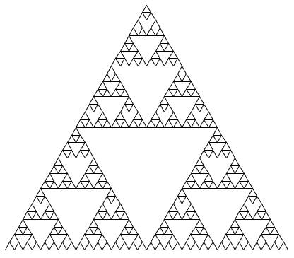
3.6.3   Structure

This section describes the general structure of a Logo interpreter. While this chapter is self-contained, it does reference the companion project. Completing that project will produce a working implementation of the interpreter sketch described here.

An interpreter for Logo can share much of the same structure as the Calculator interpreter. A parser produces an expression data structure that is interpreted by an evaluator. The evaluation function inspects the form of an expression, and for call expressions it calls a function to apply a procedure to some arguments. However, there are structural differences that accommodate Logo's unusual syntax.

Lines. The Logo parser does not read a single expression, but instead reads a full line of code that may contain multiple expressions in sequence. Rather than returning an expression tree, it returns a Logo sentence.

The parser actually does very little syntactic analysis. In particular, parsing does not differentiate the operator and operand subexpressions of call expressions into different branches of a tree. Instead, the components of a call expression are listed in sequence, and nested call expressions are represented as a flat sequence of tokens. Finally, parsing does not determine the type of even primitive expressions such as numbers because Logo does not have a rich type system; instead, every element is a word or a sentence.

>>> parse_line('print sum 10 difference 7 3')
['print', 'sum', '10', 'difference', '7', '3']

The parser performs so little analysis because the dynamic character of Logo requires that the evaluator resolve the structure of nested expressions.

The parser does identify the nested structure of sentences. Sentences within sentences are represented as nested Python lists.

>>> parse_line('print sentence "this [is a [deep] list]')
['print', 'sentence', '"this', ['is', 'a', ['deep'], 'list']]

A complete implementation of parse_line appears in the companion projects as logo_parser.py.

Evaluation. Logo is evaluated one line at a time. A skeleton implementation of the evaluator is defined in logo.py of the companion project. The sentence returned from parse_line is passed to the eval_line function, which evaluates each expression in the line. The eval_line function repeatedly calls logo_eval, which evaluates the next full expression in the line until the line has been evaluated completely, then returns the last value. The logo_eval function evaluates a single expression.

The logo_eval function evaluates the different forms of expressions that we introduced in the last section: primitives, variables, definitions, quoted expressions, and call expressions. The form of a multi-element expression in Logo can be determined by inspecting its first element. Each form of expression as its own evaluation rule.

1. A primitive expression (a word that can be interpreted as a number, True, or False) evaluates to itself.
2. A variable is looked up in the environment. Environments are discussed in detail in the next section.
3. A definition is handled as a special case. User-defined procedures are also discussed in the next section.
4. A quoted expression evaluates to the text of the quotation, which is a string without the preceding quote. Sentences (represented as Python lists) are also considered to be quoted; they evaluate to themselves.
5. A call expression looks up the operator name in the current environment and applies the procedure that is bound to that name.

A simplified implementation of logo_apply appears below. Some error checking has been removed in order to focus our discussion. A more robust implementation appears in the companion project.

>>> def logo_eval(line, env):
        """Evaluate the first expression in a line."""
        token = line.pop()
        if isprimitive(token):
            return token
        elif isvariable(token):
            return env.lookup_variable(variable_name(token))
        elif isdefinition(token):
            return eval_definition(line, env)
        elif isquoted(token):
            return text_of_quotation(token)
        else:
            procedure = env.procedures.get(token, None)
            return apply_procedure(procedure, line, env)

The final case above invokes a second process, procedure application, that is expressed by a function apply_procedure. To apply a procedure named by an operator token, that operator is looked up in the current environment. In the definition above, env is an instance of the Environment class described in the next section. The attribute env.procedures is a dictionary that stores the mapping between operator names and procedures. In Logo, an environment has a single such mapping; there are no locally defined procedures. Moreover, Logo maintains separate mappings, called separate namespaces, for the the names of procedures and the names of variables. A procedure and an unrelated variable can have the same name in Logo. However, reusing names in this way is not recommended.

Procedure application. Procedure application begins by calling the apply_procedure function, which is passed the procedure looked up by logo_apply, along with the remainder of the current line of code and the current environment. The procedure application process in Logo is considerably more general than the calc_apply function in Calculator. In particular, apply_procedure must inspect the procedure it is meant to apply in order to determine its argument count n, before evaluating n operand expressions. It is here that we see why the Logo parser was unable to build an expression tree by syntactic analysis alone; the structure of the tree is determined by the procedure.

The apply_procedure function calls a function collect_args that must repeatedly call logo_eval to evaluate the next n expressions on the line. Then, having computed the arguments to the procedure, apply_procedure calls logo_apply, the function that actually applies procedures to arguments. The call graph below illustrates the process.

The final function logo_apply applies two kinds of arguments: primitive procedures and user-defined procedures, both of which are instances of the Procedure class. A Procedure is a Python object that has instance attributes for the name, argument count, body, and formal parameters of a procedure. The type of the body attribute varies. A primitive procedure is implemented in Python, and so its body is a Python function. A user-defined (non-primitive) procedure is defined in Logo, and so its body is a list of lines of Logo code. A Procedure also has two boolean-valued attributes, one to indicated whether it is primitive and another to indicate whether it needs access to the current environment.

>>> class Procedure():
        def __init__(self, name, arg_count, body, isprimitive=False,
                     needs_env=False, formal_params=None):
            self.name = name
            self.arg_count = arg_count
            self.body = body
            self.isprimitive = isprimitive
            self.needs_env = needs_env
            self.formal_params = formal_params

A primitive procedure is applied by calling its body on the argument list and returning its return value as the output of the procedure.

>>> def logo_apply(proc, args):
        """Apply a Logo procedure to a list of arguments."""
        if proc.isprimitive:
            return proc.body(*args)
        else:
            """Apply a user-defined procedure"""

The body of a user-defined procedure is a list of lines, each of which is a Logo sentence. To apply the procedure to a list of arguments, we evaluate the lines of the body in a new environment. To construct this environment, a new frame is added to the environment in which the formal parameters of the procedure are bound to the arguments. The important structural aspect of this process is that evaluating a line of the body of a user-defined procedure requires a recursive call to eval_line.

Eval/apply recursion. The functions that implement the evaluation process, eval_line and logo_eval, and the functions that implement the function application process, apply_procedure, collect_args, and logo_apply, are mutually recursive. Evaluation requires application whenever a call expression is found. Application uses evaluation to evaluate operand expressions into arguments, as well as to evaluate the body of user-defined procedures. The general structure of this mutually recursive process appears in interpreters quite generally: evaluation is defined in terms of application and application is defined in terms of evaluation.

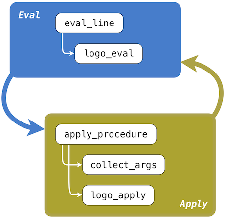
This recursive cycle ends with language primitives. Evaluation has a base case that is evaluating a primitive expression, variable, quoted expression, or definition. Function application has a base case that is applying a primitive procedure. This mutually recursive structure, between an eval function that processes expression forms and an apply function that processes functions and their arguments, constitutes the essence of the evaluation process.

3.6.4   Environments

Now that we have described the structure of our Logo interpreter, we turn to implementing the Environment class so that it correctly supports assignment, procedure definition, and variable lookup with dynamic scope. An Environment instance represents the collective set of name bindings that are accessible at some point in the course of program execution. Bindings are organized into frames, and frames are implemented as Python dictionaries. Frames contain name bindings for variables, but not procedures; the bindings between operator names and Procedure instances are stored separately in Logo. In the project implementation, frames that contain variable name bindings are stored as a list of dictionaries in the _frames attribute of an Environment, while procedure name bindings are stored in the dictionary-valued procedures attribute.

Frames are not accessed directly, but instead through two Environment methods: lookup_variable and set_variable_value. The first implements a process identical to the look-up procedure that we introduced in the environment model of computation in Chapter 1. A name is matched against the bindings of the first (most recently added) frame of the current environment. If it is found, the value to which it is bound is returned. If it is not found, look-up proceeds to the frame that was extended by the current frame.

The set_variable_value method also searches for a binding that matches a variable name. If one is found, it is updated with a new value. If none is found, then a new binding is created in the global frame. The implementations of these methods are left as an exercise in the companion project.

The lookup_variable method is invoked from logo_eval when evaluating a variable name. The set_variable_value method is invoked by the logo_make function, which serves as the body of the primitive make procedure in Logo.

>>> def logo_make(symbol, val, env):
        """Apply the Logo make primitive, which binds a name to a value."""
        env.set_variable_value(symbol, val)

With the addition of variables and the make primitive, our interpreter supports its first means of abstraction: binding names to values. In Logo, we can now replicate our first abstraction steps in Python from Chapter 1:

? make "radius 10
? print 2 * :radius
20

Assignment is only a limited form of abstraction. We have seen from the beginning of this course that user-defined functions are a critical tool in managing the complexity of even moderately sized programs. Two enhancements will enable user-defined procedures in Logo. First, we must describe the implementation of eval_definition, the Python function called from logo_eval when the current line is a definition. Second, we will complete our description of the process in logo_apply that applies a user-defined procedure to some arguments. Both of these changes leverage the Procedure class defined in the previous section.

A definition is evaluated by creating a new Procedure instance that represents the user-defined procedure. Consider the following Logo procedure definition:

? to factorial :n
> output ifelse :n = 1 [1] [:n * factorial :n - 1]
> end
? print fact 5
120

The first line of the definition supplies the name factorial and formal parameter n of the procedure. The line that follows constitute the body of the procedure. This line is not evaluated immediately, but instead stored for future application. That is, the line is read and parsed by eval_definition, but not passed to eval_line. Lines of the body are read from the user until a line containing only end is encountered. In Logo, end is not a procedure to be evaluated, nor is it part of the procedure body; it is a syntactic marker of the end of a procedure definition.

The Procedure instance created from this procedure name, formal parameter list, and body, is registered in the procedures dictionary attribute of the environment. In Logo, unlike Python, once a procedure is bound to a name, no other definition can use that name again.

The logo_apply function applies a Procedure instance to some arguments, which are Logo values represented as strings (for words) and lists (for sentences). For a user-defined procedure, logo_apply creates a new frame, a dictionary object in which the the keys are the formal parameters of the procedure and the values are the arguments. In a dynamically scoped language such as Logo, this new frame always extends the current environment in which the procedure was called. Therefore, we append the newly created frame onto the current environment. Then, each line of the body is passed to eval_line in turn. Finally, we can remove the newly created frame from the environment after evaluating its body. Because Logo does not support higher-order or first-class procedures, we never need to track more than one environment at a time throughout the course of execution of a program.

The following example illustrates the list of frames and dynamic scoping rules that result from applying these two user-defined Logo procedures:

? to f :x
> make "z sum :x :y
> end
? to g :x :y
> f sum :x :x
> end
? g 3 7
? print :z
13

The environment created from the evaluation of these expressions is divided between procedures and frames, which are maintained in separate name spaces. The order of frames is determined by the order of calls.

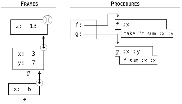
3.6.5   Data as Programs

In thinking about a program that evaluates Logo expressions, an analogy might be helpful. One operational view of the meaning of a program is that a program is a description of an abstract machine. For example, consider again this procedure to compute factorials:

? to factorial :n
> output ifelse :n = 1 [1] [:n * factorial :n - 1]
> end

We could express an equivalent program in Python as well, using a conditional expression.

>>> def factorial(n):
        return 1 if n == 1 else n * factorial(n - 1)

We may regard this program as the description of a machine containing parts that decrement, multiply, and test for equality, together with a two-position switch and another factorial machine. (The factorial machine is infinite because it contains another factorial machine within it.) The figure below is a flow diagram for the factorial machine, showing how the parts are wired together.

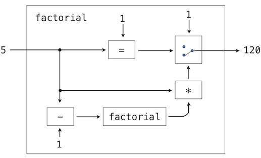
In a similar way, we can regard the Logo interpreter as a very special machine that takes as input a description of a machine. Given this input, the interpreter configures itself to emulate the machine described. For example, if we feed our evaluator the definition of factorial the evaluator will be able to compute factorials.

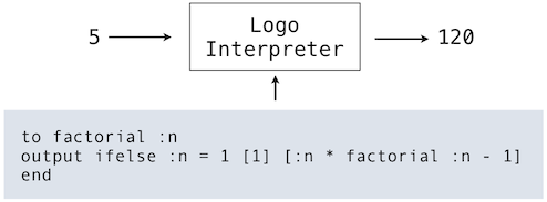
From this perspective, our Logo interpreter is seen to be a universal machine. It mimics other machines when these are described as Logo programs. It acts as a bridge between the data objects that are manipulated by our programming language and the programming language itself. Image that a user types a Logo expression into our running Logo interpreter. From the perspective of the user, an input expression such as sum 2 2 is an expression in the programming language, which the interpreter should evaluate. From the perspective of the Logo interpreter, however, the expression is simply a sentence of words that is to be manipulated according to a well-defined set of rules.

That the user's programs are the interpreter's data need not be a source of confusion. In fact, it is sometimes convenient to ignore this distinction, and to give the user the ability to explicitly evaluate a data object as an expression. In Logo, we use this facility whenever employing the run procedure. Similar functions exist in Python: the eval function will evaluate a Python expression and the exec function will execute a Python statement. Thus,

>>> eval('2+2')
4

and

>>> 2+2
4

both return the same result. Evaluating expressions that are constructed as a part of execution is a common and powerful feature in dynamic programming languages. In few languages is this practice as common as in Logo, but the ability to construct and evaluate expressions during the course of execution of a program can prove to be a valuable tool for any programmer.