A. Intro

Download the code for Lab 26 and create a new Eclipse project out of it.

Learning Goals

Over the summer, we have covered all of the fundamental ADTs and the most common implementations of them. In today's (the final) lab, we will go over two more data structures that can be used to implement ADTs as well as a completely new ADT. First we will go over splay trees, another type of balanced tree. Then we'll study Disjoint Sets and Kruskal's Algorithm, which uses Disjoint Sets. Finally we will cover a new way to hash, cuckoo hashing.

B. Splay Trees

As we have seen before, when dealing with search trees, we like to have them balanced in order to keep the runtime of the basic operations, like insertion, deletion, and finding, in O(lg n) time, where n is the number of items in the search trees. We introduced the AVL tree, which kept balance by adding an extra invariant about its height. This time however, we will not even care about height. Not explicitly at least, and yet we'll still be "balanced".

What?! How is that possible. If we do not keep an invariant on height somehow, then how can we have balance? Well, it is possible, and the data structure that does this is called a splay tree. A splay tree is just a regular BST, except it has a little twist to its basic algorithms for insert, removal, and finding.

All operations in a splay tree will end by splaying the last node accessed up to the root. What is splaying? It's just a series of tree rotations! Just like an AVL tree, a splay tree maintains its "balance" by rotations. Splaying the latest accessed node will make sure that the tree is reasonably balanced, as well as giving the splay tree a key advantage over AVL trees, which is that splay trees have fast access to things that have been accessed recently. Things that have been accessed recently will be by the root. That means that if you keep accessing the same items a lot of times, you will be able to get them quickly!

There are three cases that occur when splaying.

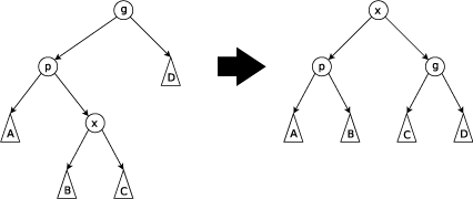
Case 1: Zig-Zag

Let's say that the node that we are splaying up, X, is the right child of a left child (or the mirror, the left child of a right child). P is the parent of X, and G is the grandparent. First we will rotate X left through P, and then rotate X right through G. The mirror case will do a right rotation first, followed by a left rotation. This is the zig-zag case, as seen below.

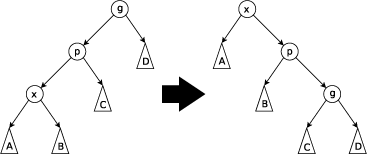
Case 2: Zig-Zig

Now let's say that X is the left child of a left child (or the mirror, right child of a right child). What we do this time, is we rotate P right through G, and then we rotate X right through P. The mirror case will rotate P left and then X left. You can see this below.

So as you see, after zig-zig-ing and zig-zag-ing, X will go up two levels at a time. Eventually what will happen is that X becomes the root! ...or it will be the child of the root, in which we bring up our third case.

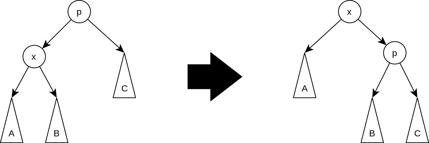
Case 3: Zig

If X's parent is the root of the entire splay tree, then we just rotate X so that it becomes the root.

Now try it for yourself. You can go here to see a visualization of splay trees in action.

One interesting thing to note about splay trees is that, it usually will not stay unbalanced for long. For example, say we had the splay tree below.

Let's say that we then do contains(1). After we find 1, we then splay it up to the root, which results in this tree.

Exercise: Zig-ing and Zag-ing

In SplayTree.java, you have been given the code for left and right rotations (after all you already did that when you coded up AVL trees). Now implement the zig(), zigZag(), and zigZig() methods, which do the rotations described in the three cases above. Afterwards, implement the splayNode() method, which is used by put() and get() in order to splay the most recently accessed node to the root of the Splay Tree. Remember your null checks!!

C. Disjoint Sets

Now we will learn about an entirely new data structure/ADT, called a Disjoint Set. The data structure represents a collections of sets, that are, well disjoint, meaning that no item is found in more than one set.

There are only two operations that disjoint sets support, and those are the find and union operations. What find does is that it takes in an Object and it tells us which set it is in. Union will take two sets and merge it into one set.

So that is all good and well, but what does that exactly mean? Well we can think of Disjoints Sets as representing companies. Disjoint Sets start with each company in its own set. Then we can call the union operation to represent a company acquiring another company.

For example, let's take these three companies.

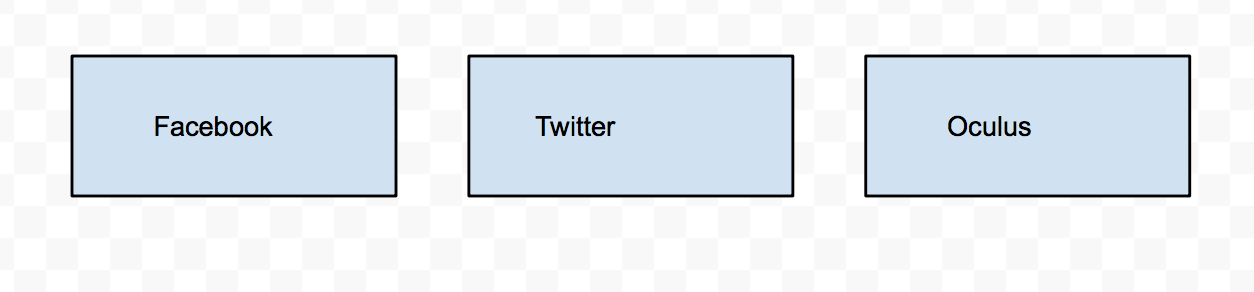
Right now, find(Facebook) will get us Facebook, find(Oculus) will get us Oculus, and find(Twitter) will get us Twitter. Now let's do union(Facebook, Oculus)

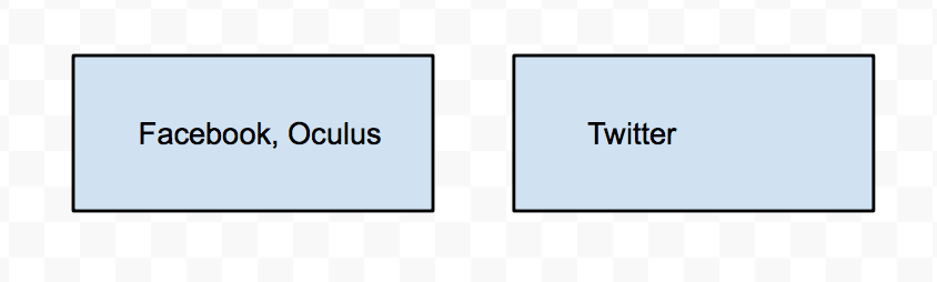
Now, find(Oculus) will give us Facebook! We have merged the two sets together.

So that is the overall idea of a Disjoint Set, the ADT for it. What about the implementation?

First, we need to decide on how to represent each of the individual sets. I am going to claim that the best way to do this through a tree, where the root of each tree will be the name of the set. Going back to our company example, it is which company is actually in charge. What does this mean for the runtime for our operations? Well union will still take O(1) time, all you need to do is take the root of one set and make it the child of another. But how about find? Well, overall they are slower, to find what set you are in, you have to travel up your parents until you get to the root. But I am going to say that prioritizing union operations will overall give us a faster data structure.

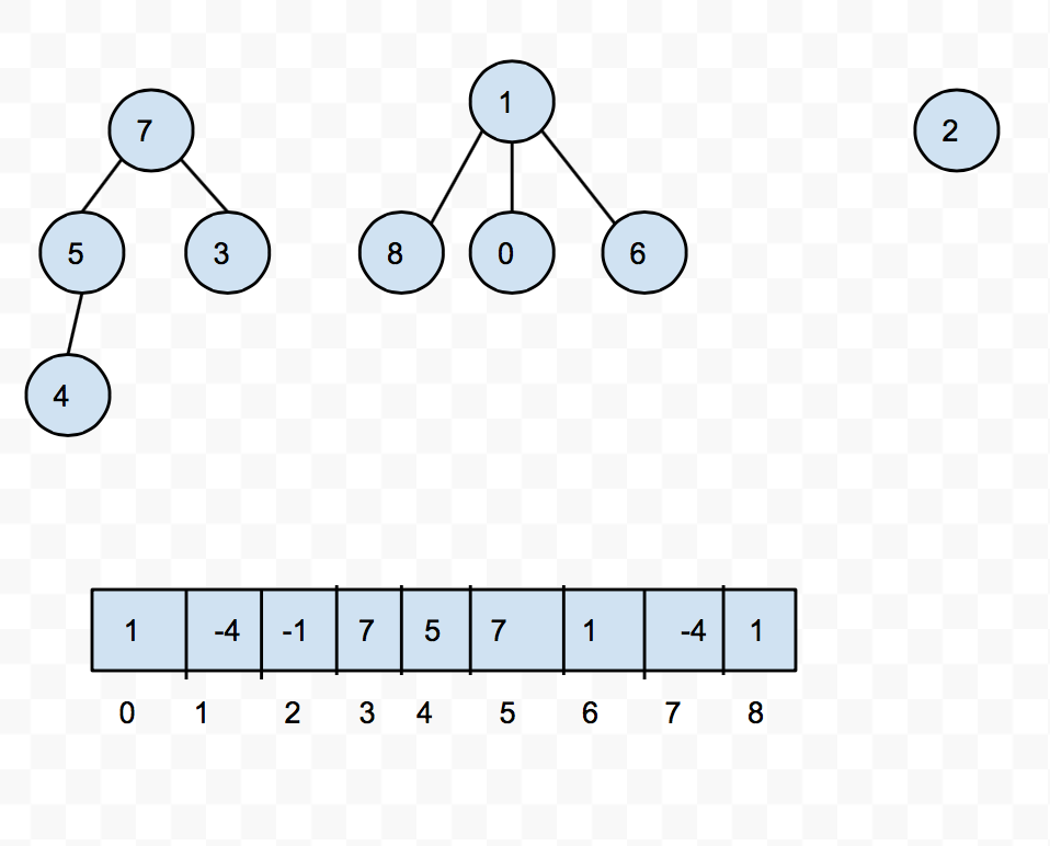
Now how exactly do we represent these trees? We can do it with an array! Let's say for a second that our Disjoint Set will only hold non-negative integers. If that is the case, then we can use an array to mark what the parent of each item is. When we get to the root of the tree, we will record the size of the set, and to distinguish it from a parent reference, we will make the size negative.

You can see this in the picture below.

So now to union two trees, all we need to do is update the reference in the array and change the size. What about find? Well what find will do is that it will keep traveling up references in the array until you get a negative number, at which point you can return the index.

Now of course to gain the best possible runtime for our data structure, we need to do some optimizations. One optimization is called union-by-size. That is, when we do union on two sets, which we are representing as trees, we will take the smaller tree and make it the subtree of the larger tree.

Another optimization is called path compression. Remember that Disjoints Sets only care about which set you are in, which is determinded by the root of the tree that represents the set. So what path compression does is that when you call find(), we will move all of the nodes that we encounter as we go to the root, children of the root. It sounds a bit confusing, but hopefully it will make sense when you see it in action.

Let's take this tree.

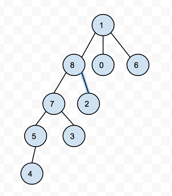
After we do find(4), path compression will leave us with a tree like this.

This is great because now calling find() on what were previously ancestors of 4 will now just take O(1) time, after all they are children of the root. And when we call find on any decendents of the previous ancestors of 4, those operations will now be faster.

So with union-by-size and path compression, we get find to be very very close to constant time. Officially, a series of u unions and f find operations will take O(u + f * alpha(f + u, u)), where alpha is what is called the inverse Ackermann function, which is an extremely slow growing function. And by extremely slow growing, I mean, it is never bigger than 4 for any standard purposes.

To play around with Disjoint Sets, you can go here. Remember to check the boxes for path compression and union-by-rank, where and have rank be the number of nodes.

D. Minimum Spanning Trees

So we have this cool data structure, but what exactly can we use it for? It looks like we can model companies buying each other out, but there's got to be something else we can do with it. And there is.

Let's take a break from disjoint sets and introduce you to a Minimum Spanning Tree. What exactly is it? Well, if we have an undirected graph G, a spanning tree of the graph is essentually something that is connected, that is it reaches all of the vertices in G, acyclic, and inclues all of the vertices. If we have weights in the graph, then we can define the minimum spanning tree as the spanning tree of G with minimum total weight, as in if you add up all of the edges in the spanning tree, that is as light as it will ever be.

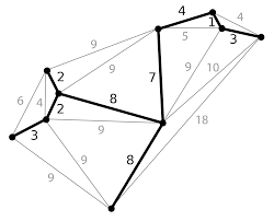
For example, here is a minimum spanning tree. You can see all of the edges that are not in the MST in gray.

There are many applications for MSTs, including network design, medical imaging, planning out electric wiringly, the list goes on and on.

E. Kruskal's Algorithm

But how can we find these MSTs. Well, we can use Kruskal's algorithm which goes like this

To find a minimum spanning tree, T of G, what we do is first

1. Make a new Graph T (which will become the MST) with the same vertices as G, no edges yet though.
2. Make a list of all of the edges in G.
3. Sort the edges by weight, from least to greatest
4. Go through the edges in sorted order, and for each edge (u,v), if there is not already a path in T from u to v, then we add the edge (u,v) to T

Sounds easy right? The actual proof for why Kruskal's algorithm works will come to you in CS170. But for now, we can at least talk about the runtime. The really tricky part for this algorithm is in step 4, determining if two vertices are already connected. A naive way to do this would be to simply use one of our graph traversal algorithms that we have learned before. But that is way too slow. How can we see if two things are already together. Through a Disjoint Set! We can have a Disjoint Set of vertices (which as you may recalled we label with integers) and as we add edges into T, we can union these vertices together. If we call find on two vertices and it ends up that they are in the same set, then they are connected and we do not add any edges.

So what is the runtime? Well if we are using an adjacency list, then it takes O(|V|) time to make the initial graph, and sorting if you recall will take O(|E| lg |E|) time. And then to iterate through all of the edges, will take O(|E|) time (plus the little inverse Ackermann factor that the Disjoint Sets bring in). So overall, Kruskal's will run in O(|V| + |E| lg |E|).

For a visualization of Kruskals, you can go here.

Excerise: Coding up Kruskal's

I have provided you an implementation of a Quick-Union Disjoint Set with path compression, as well as a weighted, undirected graph implementation (courtesy of Princeton). Take a second to see how they work and then in Kruskals.java implement the mst() method, which takes in an EdgeWeightedGraph and returns a new EdgeWeightedGraph, which is an MST of the input graph.

F. Cuckoo Hashing

So far, we have seen two types of hashing schemes, chaining and linear probing. Now we will introduce a third way to hash!

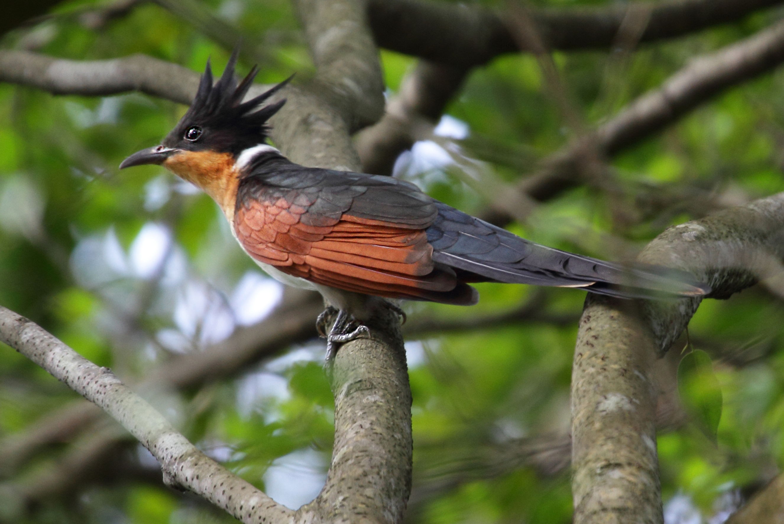
The scheme is called cuckoo hashing, named after this bird.

So what is cuckoo hashing? Well the idea is pretty simple. Instead of having one array, we will keep two of them, both of the same length, and each array will have a different compression function. That is two different ways of figuring out which index to store the key-value pair. In this class, we have mainly been dealing with one compression function, which is simply to mod the hashCode by the length of the array. Cuckoo hashing requires you to have two different compression functions, that are probably more fancy than just taking the mod.

So we have two arrays, so what? Well, It starts off like normal hashing, you get the hashCode of the key, compress it, and then put it in the right spot in the array. The twist is when we have a collision. If something is already at the index, then we evict from the current array, and then rehash in our second array! (That is where the name cuckoo hashing comes from, some species of cuckoo birds push other eggs/young other of the nest when they hash).

This is great! No need to worry about chaining, and there can only be two places where any item can be, in one array or the other. There is one slight caveat though. What happens when as you are rehashing things, you end up in a cycle, and keep rehashing the same things over and over and over again.

Good news is, we can handle that! What we do, is we set a limit to now many times we will rehash items. Once we pass that limit, then we just give up, and we rehash everything! Usually we either pick new compression functions, or we do our standard schema and double the size of both arrays and rehash.

Cuckoo hashing is great because of the fact that we get an actual guarantee for a constant time lookup. Although we do have to do more work for insertions, we can prove that on average insertion will take O(1) time. The exact proof for this however is beyond the scope of this course and requires some intense graph theory knowledge and probability. In practice, cuckoo hashing actually works pretty well.

You can look to see how exactly cuckoo hashing works here

G. Conclusion

As lab26, please turn in SplayTree.java and Kruskals.java