Introduction
This document contains a simplified explanation of how neural networks work. Each section contains a high-level explanation followed by relevant pieces of code from the matrix version of Project 4. The code is hidden by default for those who just want the big ideas, but I recommend that you press "Show Code" and read through the code snippets so that the explanations make more sense. Since this a simplified explanation, this document may contain slight inaccuracies. However, it should provide a starting point for further exploration should you find the topic interesting. If you have any questions or comments, please post them in the corresponding Piazza thread.
Making Decisions with Machines
Suppose you are trying out a new restaurant in town. You may evaluate the restaurant on a few factors, such as the quality of food, the price, and the service. Not all factors are equally important--if the food tastes disgusting, no matter how good the service was you would never go there again. In the end, you might label the restaurant as "great", "mediocre", or "avoid like the plague". This is an example of a classification problem, where given a list of factors, you assign a class to that input.
In machine learning, each factor is known as a feature. Given a list of features, we can make a decision by scaling each feature by a weight reflecting the feature's importance, and then somehow combining the weighted features to form a smaller set of values which we then interpret. For classification problems, each value in the set often reflects the likelihood of the input being of a certain class, so we can assign the class associated with the maximum value as our output. We have thus sketched a classifier for our problem.
A classifier cannot classify well without an appropriate choice of weights, but it is often infeasible to manually determine what the weights should be. In machine learning, we expose the classifier to reference input/output pairs (called the training set). For each example in the training set, the classifier first makes a classification based on the current weights, and then updates the weights based on how "different" the predicted result is from the expected result. The function used to calculate the differentness is known as the loss function. This process repeats until some stopping criteria is reached.
The Linear Classifier
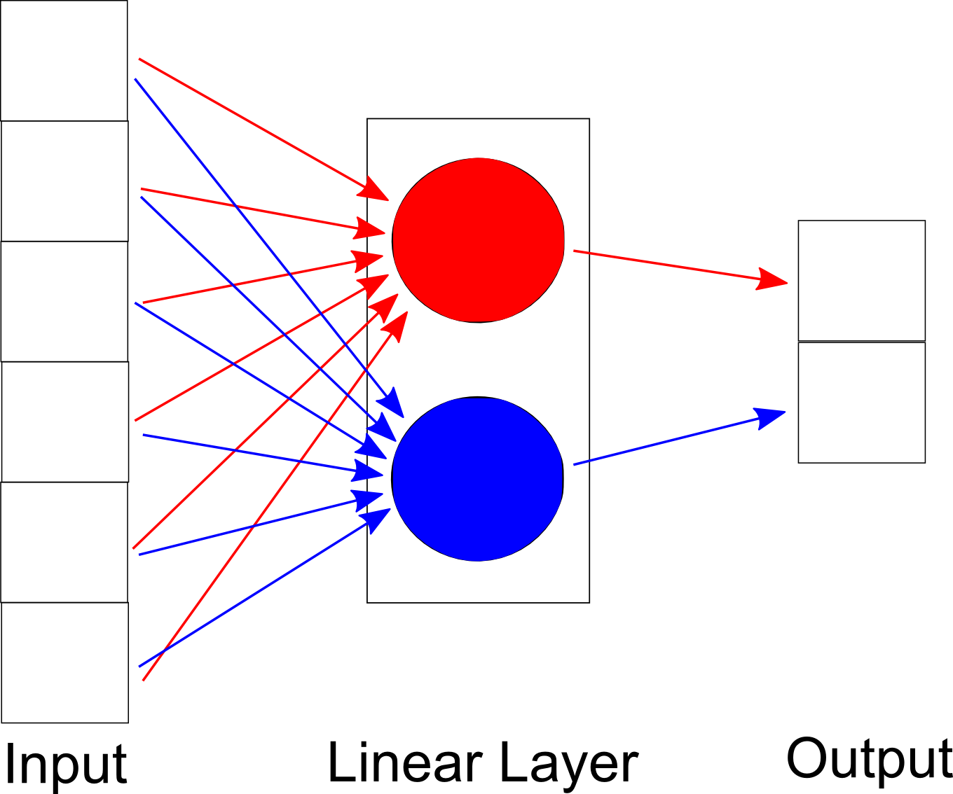
We mentioned that features are scaled by weights and then combined, but we did not specify how they are combined. One of the simplest methods is to add them up. If x0, x1, ..., xk are the features, and w0, w1, ..., wk are the corresponding weights and b is a constant, we are computing the linear function: y = x0 * w0 + x1 * w1 + ... + xk * wk + b.
Linear classifiers often contain more than one such function. For example, our linear classifier has one per output class, and more complicated classifiers can have many more. However, each function uses the same set of inputs, and therefore they exist on the same "level". You can imagine each function as being part of a node, which together forms a layer. This particular layer is a linear layer since it performs linear operations.
During training, the output of the linear layer is compared with the expected output using our loss function. The loss function can be used to find the loss function's gradient, or how much we should change our predicted output to match the expected output. But what we really want to know is how much we should change our weights. It turns out we can treat a layer as a mathematical function, which means that we can write the output of the linear layer a function of the input and its weights. Since we know how much the output should change, we can calculate how much the each weight should change by taking the derivative with respect to each weight. This is done in the backwards pass and forms the backbone of classifier training. (Side note: typically weights aren't changed by the derivative itself, but by an amount that depends on the derivative.)
Neural Networks
Unfortunately, the linear layer is restrictive. For example, suppose we used a classifier to pick our next vacation spot, and one of the features was distance from home. A location that was 300 miles away and a spot that was 3000 miles away would both be considered far, and qualitatively the two wouldn't be too different. However, a linear classifier would consider the latter feature to be 10x more different, which could skew the results.
The solution is to introduce nonlinearity into our classifier. To do so, we use activation functions, which transforms its input a non-linear fashion. Our neural net contains three layers (remember that each layer contains multiple nodes):
- A linear layer
- A layer using the rectifier activation function (called rectified linear unit, or ReLU)
- A second linear layer

The layers are chained, meaning the ouput of layer 1 is fed into layer 2, and the output of layer 2 is fed into layer 3. This makes the weight update step, which involves taking derivatives, a bit more complicated. While the change in layer 3 depends on the gradient of the loss function, the change in layer 2 depends on the gradient of layer 3, and the change in layer 1 depends on the gradient of layer 2. Mathematically speaking, this is simply the chain rule of calculus. Since the gradients propagate from the end of the classifier to the beginning, this process is called backpropagation.
(Side note: In neural network literature, each unit is referred to as a "neuron", and each neuron contains both a linear component and an activation function, so this network would be referred to as a two-layer neural network.)
Convolutional Neural Networks
In theory, neural network of sufficient size as described above can model any function. However, the amount of time and data needed to train such a network makes them utterly impractical. The reason is that each node in a layer uses all nodes from the previous layer as inputs, so the number of weights grow very quickly as the neural net increases in size.
One approach that combats this issue is convolutional neural networks. In a convolutional neural network, each node is not connected to the entire previous layer. Rather, the node uses only a few nodes from the previous layer as input, greatly reducing the number of parameters. During the forward pass, the node performs a convolution with the input, which basically "sweeps" the node across the input.
You don't need to know the details about convolution. What is important to know is that convolution acts as a filter (think Photoshop) on an input. Depending on the weights of the node, also called the kernel in this context, a convolution can perform operations like shape detection, edge detection, blurring, sharpening, etc. A convolutional neural net uses the training set to learn the set of filters needed for the classification task.
A collection of nodes, or kernels, acting on the input forms a convolution layer. The output of the convolution layer is then passed to an activation layer (in this case, a ReLU layer). However, convolution produces a large output, which is undesirable. We thus introduce a pool layer after the activation layer to downsize our output.
The sequence of convolution, activation, and pool layers can be chained together. Backpropagation happens in the same way as before, with the gradient of the kth layer used to caculate the gradient of the k-1th layer.
Further Reading
- Neural Networks and Deep Learning
- A Course in Machine Learning, chapters on perceptrons (linear classifiers) and neural networks.
If you are interested in this topic, take CS 188 and CS 189!