Introduction
In this project we will use the ns-2 network simulator to
evaluate variants of TCP and optimize their parameters based on ns-2
simulations.
This project has to be done in groups of 3.
Deadlines
There are three phases in the project. A report will be due at the end of each phase.
- Phase I is due on Thursday, March 9.
Instructions
Phase I
In this phase we will get
familiar with running basic ns-2 simulations. We will evaluate the following
flavors of TCP -- Tahoe,
- Consider the following
network topology.
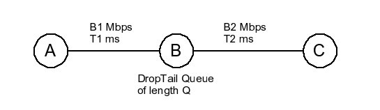
There is an FTP connection (which uses TCP) from node A to node C which starts at time t=0s. Assume that each packet is 1250 bytes in length. - Set B1=25, B2=10,
T1=10, T2=20, Q=10. Simulate the FTP transfer for 50s for each of TCP
"Tahoe", TCP "
- Plot the congestion window for each of the TCP flavors as a function of time on the same graph.
- Compute the achieved throughput for each of the TCP flavors and compare them against each other. Explain why one of them does better than the other in terms of achieved throughput. How do these results compare with the maximum achievable throughput?
- Set B1=30, B2=20,
T1=10, T2=200, Q=125. Simulate the FTP transfer for 2000s for TCP "
- Plot the congestion window for both the TCP flavors as a function of time on the same graph.
- Compute the achieved throughput for each of the TCP flavors and compare them against each other. Explain why one of them does better than the other in terms of achieved throughput.
- We now consider the topology
shown below.
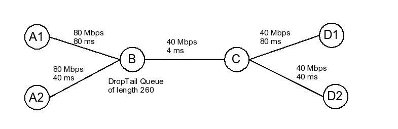
There is an FTP/TCP flow from A1 to D1 and another from A2 to D2. Note that the propagation delay from A1 to D1 is twice as large as the propagation delay from A2 to D2. Assume that each packet is 1250 bytes in length. Consider the following scenarios: - Suppose both the flows: A1->D1, A2->D2 use TCP "Tahoe". Both the flows start at time t=0s. Run the simulation for 1500s. Plot the congestion windows for both the flows as a function of time on the same graph. What are the achieved throughputs for each of these flows? Does each flow get a fair share of the bandwidth? Why or why not? By how much do the throughputs for the flows differ? Explain.
- Repeat part (a) with
both flows using TCP "
- Repeat part (a) with both flows using TCP "Vegas".
- Repeat part (a) with both flows using TCP "FAST".
Tips
- Avoid using the trace-all/namtrace-all feature for long simulations -- it will fill up your disk quota.
- For all simulations, set window_ variable for all TCP agents to 100000 to ensure that the receiver window size does not become a bottleneck.
- You have to use Agent/TCP/Fast. There is no NS documentation. But you can visit http://www.cubinlab.ee.mu.oz.au/ns2fasttcp/ and http://netlab.caltech.edu/FAST/ for more info on FAST TCP. There are a few test scripts on the first site that you could possibly use.
Project Submission
Phase I
Submit a report along with the ns-2 scripts used together in a single tar file. Email the tar file to ee122-ta@imail.eecs.berkeley.edu, ee122-tb@imail.eecs.berkeley.edu with the subject line as "EE122 Project Phase I" by 11.59pm, Thursday March 9.
Resources
- ns-2 is installed on the instructional machines under /share/instsww/pkg/ns-allinone-2.27-fasttcp. To run it from your account make sure to add /share/instsww/ns-allinone-2.27-fasttcp/bin to the PATH environment variable and /usr/sww/lib to the LD_LIBRARY_PATH variable.
- ns-2 online documentation is here.
- gnuplot is a good tool for generating plots. You will find useful links here.
Phase I Clarifications:
1. For Question 1: Note that throughout
this question, there is only ONE TCP flow. So, in part (a), you will run the
setup using TCP Tahoe for 50s. Then you will run another simulation using TCP
Reno for 50s. And in the end of part (a), you will run the same setup using TCP
Vegas for 50s. For part (b), you run one simulation using the same setup with
TCP Reno and then another simulation for TCP FAST.
2. For both questions 1 and 2, you will
need to plot congestion windows as a function of time. Since the simulations
run for a long time, your plots will not be very clear. So, for plotting
congestion windows, please plot the windows upto a
small enough time (a good suggestion is when TCP Reno reaches its peak window
size 6 times) to illustrate the differences between the different flavors of
TCP.
3. The cwnd_ variable for a tcp
agent is the congestion window size in number of packets.
4. The ack_ and maxseq_
variables for a tcp agent are also in number of
packets (NOT number of bytes). ack_
stores the last packet for which the ack was received
by the sender. maxseq_ stores
the highest numbered packet sent by the sender.