Lab 6, Digital Communication with Audio Frequency Shift Keying (AFSK)
In this part of the lab we are going to experiment with Digital modulation and communication. Network Communication systems have layered architechture. The bottom layer is the physical which implements the modulation. Here we will use AFSK, which is a form of BFSK in the audio range (hence the 'A'). We will write a modulator/demodulator for AFSK. In the following part of lab we will leverage AX.25, which is an amateur-radio data-link layer protocol. AX.25 is a packet based protocol that will help us transmit data using packets. It implements basic synchronization, addressing, data encapsulation and some error detection. In the ham world, an implementation of AFSK and AX.25 together is also called a TNC ( Terminal Node Controller ). In the past TNC's were separate boxes that hams used to attach to their radios to communicate with packet-based-communication. Today, it is easy to implement TNC's in software using the computer's soundcard.... as you will see here!
%pylab
# Import functions and libraries
import numpy as np
import matplotlib.pyplot as plt
import pyaudio
import Queue
import threading,time
import sys

from numpy import pi
from numpy import sin
from numpy import zeros
from numpy import r_
from scipy import signal
from scipy import integrate

import threading,time
import multiprocessing

from rtlsdr import RtlSdr
from numpy import mean
from numpy import power
from numpy.fft import fft
from numpy.fft import fftshift
from numpy.fft import ifft
from numpy.fft import ifftshift
import bitarray
from  scipy.io.wavfile import read as wavread
import serial

%matplotlib inline
AFSK1200, or Bell 202 modem
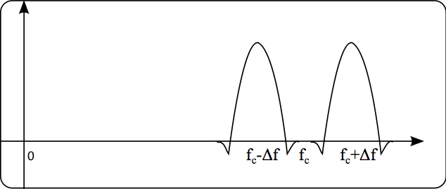
AFSK1200 encodes digital binary data at a data-rate of 1200b/s. It uses the frequencies 1200Hz and 2200Hz ( center frequency of $1700$Hz $\pm 500$ Hz) to encode the '0's and '1's (also known as space and mark) bits. Even though it has a relatively low bit-rate it is still the dominant standard for amature packet radio over VHF. It is a common physical layer for the AX.25 packet protocol and hence a physical layer for the Automatic Packet Reporting System (APRS), which we will describe later.
The exact frequency spectrum of a general FSK signal is difficult to obtain. But, when the mark and space frequency difference $\Delta f$ is much larger than the bit-rate, $B$, then the bandwidth of FSK is approximately $2\Delta f + B$. This is not exactly the case for AFSK1200 where the spacing between the frequencies is 1000Hz and the bit-rate is 1200 baud.
Note, that for the (poor) choice of 1200/2200Hz for frequencies, a synchronous phase (starting each bit with the same phase) is not going to be continuous. For the Bandwidth to be narrow, it is important that the phase in the modulated signal is continuous. For this reason, AFSK1200 has to be generated in the following way: $$ s(t) = cos\left(2\pi f_c t + 2\pi \Delta f \int_{\infty}^t m(\tau)d\tau \right),$$ where $m(t)$ has the value =1 for a duration of a mark bit, and a value =-1 for a duration of a space bit. Such $m(t)$ signal is called an Non-Return-to-Zero (NRZ) signal in the digital communication jargon. Here's a link to some notes provided by Fred Nicolls from the university of Cape Town
The integration guarentees that the phase in continuous. In addition, the instantaneous frequency of $s(t)$ is the derivative of its phase, which is $2\pi f_c + 2\pi \Delta f m(t)$, which is exactly what we need.
Write a function
sig = afsk1200(bits)the function will take a bitarray of bits and will output an AFSK1200 modulated signal of them, sampled at 44100Hz. Note that Mark frequency is 1200Hz and Space Frequency is 2200Hz. If your USB device prefers 48000Hz, then use 48KHz for the sampling rate.Note, that 44100 does not divide by 1200 so each "bit" will have non-integer length in samples. If you are not careful, this would lead to deviation from the right rate over time. To make sure that you produce signals that have the right rate over time generate the signal first at a rate of 44100*4 (which does divide by 1200) for the entire bit sequence and then downsample by 4 at the end. You don't need to low-pass filter, since the signal is narrow banded anyways.
For integration, use the function integrate.cumtrapz, which implements the trapezoid method.
def afsk1200(bits):
    #the function will take a bitarray of bits and will output an AFSK1200 modulated signal of them, sampled at 44100Hz
    fs = 44100*4


    #your code here


    sig = real(exp(1j*ph[::4]))
    return sig
- Generate a sequence of 64 randomly generated bits with equal probability. Generate the AFSK1200 signal and compute its spectrum.
- Does the spectrum looks like the one in Figure 2?
bits=bitarray.bitarray((rand(64)>0.5).tolist())
sig = afsk1200(bits)
fig = figure(figsize(16,4))
plot(linspace(0,22050/4,20000/4),abs(np.fft.fft(sig,n=40000))[:20000/4])

xlabel('Hz')
title('Spectrum of AFSK1200')
AFSK1200 demodulation
AFSK is a form of digital frequency modulation. As such it can be demodulated like FM. Because AFSK alternates between two frequencies, we can place two bandpass filters around the frequency of the Mark and Space and use envelope detection to determine which frequency is active in a bit period. This is a non-coherent AFSK demodulation, because the receiver phase does not need to be synced to the transmitter phase in order to demodulate the signal. The implementation we will use here is loosly based on on the one by Sivan Tolede (4X6IZ), a CS faculty in Tel-Aviv university who has written a nice article on a high-performance AX.25 modem. You can find it Here.
Non-Coherent Demodulation of AFSK
Here's a diagram of a non-coherent AFSK1200 demodulator that returns an NRZ signal:
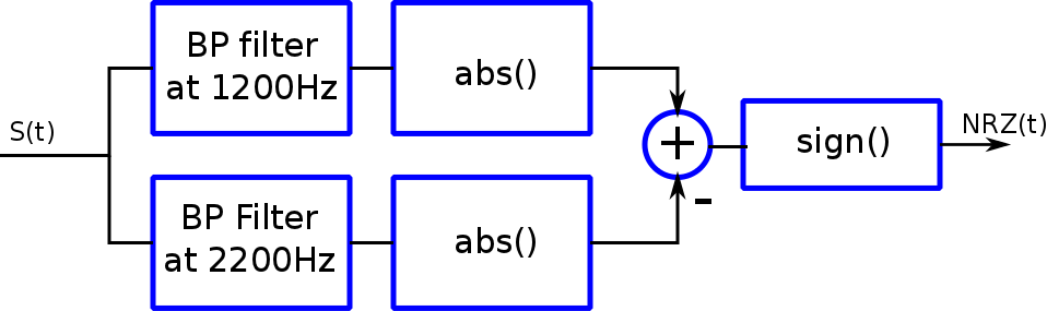
- Using signal.firwin design a TBW=2 LP filter with a (two-sided) bandwidth of approximately 1200Hz for a sampling rate of 44100Hz.
- From the LP filter gernerate two bandpass filters by complex modulating the LP filter to be centered around 1200Hz and 2200Hz respectively.
- Filter the random stream of bits you generated previously using the two filters.
- The absolute value of the result represents the envelope of the filtered signal. The difference between the envelopes should represent the NRZ signal. Display the difference between the envelope of the resulting two signals. Can you see the bits?
# Generate filters
TBW = 2
N =
BW =
h_space =
h_mark =
print(BW)
# plot the magitude impulse response of the space filter

figure
plot(abs(h_space))
# Filter the signal and compute the difference between the envelopes of the results use signal.fftconvolve
# plot the resulting difference NRZa

# your code here:


NRZa =
- Extract the digital NRZ signal by computing the signum (
sign) function of the difference. - The bit value is the value of the NRZ function in the middle of the bit period. Decode the bits and compare to the original ones. Don't forget to compensate for the delay of the filter. Overlay a stem plot on top of the NRZ signal at the indexes in which you sampled the bit values. Make sure as a sanity check that you actually sampled at the middle of the interval.
# your code here.
FM demodulation of AFSK
We can also demodulate AFSK using FM demodulation. Recall that the bandwidth of AFSK is approximately $2\Delta f + B$ where $B$ is the bitrate (1200Hz for AFSK1200). The afsk signal is $s(t) = cos\left(2\pi f_c t + 2\pi \Delta f \int_{\infty}^t m(\tau)d\tau \right)$. If we filter the signal by passing only the positive frequencies we will get $s(t) = \frac{1}{2}e^{2\pi j f_c t + 2\pi j \Delta f \int_{\infty}^t m(\tau)d\tau}$. This is the analytic signal and we can FM demodulate it in a similar way as we did for the FM radio Lab by taking the derivative of the phase. After appropriate scaling and offset we can extract the NRZ signal.
- Design a low-pass filter with the appropriate BW to cover the entire FSK spectrum (both mark and space, or $2\Delta f + B$)
- Complex modulate the LP filter to create a BP filter centered around 1700Hz.
- Use the BP filter to get the analytic signal.
- FM demodulate the signal, scale and offset the signal appropriately to get the "analog" NRZ signal of approximately $\pm 1$
- Optional: Low-pass filter the signal with a cutoff frequency of 1200Hz to reduce demodulation noise.
- Remember that '1' is the 1200Hz frequency and '0' is 2200.
- rectify the resulting NRZ by taking the signum function of it.
- make a plot similar to the non-coherent asfk demodulation
# your code here
- Write a function nc_afskDemod(sig, TBW=TBW, N=Nfilter) that implements the above non-coherent demodulation and returns the "analog" NRZ (i.e. without rectifying it). You can assume that the sampling rate is 44100Hz (or 48000 if you used that rate before)
- Write another function fm_afskDemod(sig, TBW=TBW, N=Nfilter) that implements the above fm demodulation and returns the "analog" NRZ (i.e. without rectifying it). You can assume that the sampling rate is 44100Hz (or 48000 if you used that rate before)
def nc_afskDemod(sig, TBW=2.0, N=74):
    #  non-coherent demodulation of afsk1200
    # function returns the NRZI (without rectifying it)

    # your code here


    return NRZI

def fm_afskDemod(sig, TBW=4, N=74):
    #  non-coherent demodulation of afsk1200
    # function returns the NRZI (without rectifying it)

    # your code here


    return NRZI
Bit Error Rate (BER)
One of the ways to evaluate the properties of a digital modulation scheme is to compute the bit-error-rate (BER) curves with as a function of signal-to-noise ratio (SNR). The BER is the number of bit errors (received bits that have been altered due to decoding error) divided by the total number of transmitted bits.
Let's calculate the BER for AFSK with both the non-coherent and FM demodulations:
- Generate a 10000 long random bitstream
- AFSK1200 modulate the bitstream
- Add random gaussiam noise with a standard deviation of 1 to the afsk signal.
- demodulate using both methods and compute the BER
- plot the first 300 samples of the ourput of the BP filters of the non-coherent demodulation and the analog NRZ of the fm demodulation to see how erros look like
# your code here
fig = figure(figsize=(16,4))
plot(NRZa[:3000])
title('result of non-coherent demodulation')

fig = figure(figsize=(16,4))
plot(NRZ_fma[:3000])
axis((0,3000,-2,2))
title('analog NRZ of fm demodulation')
# compute bit error rate
Your Bit error rate will depend also on the quality of the reconstruction. You can try to repeat the experiment for different choices of filters if you like.
Computing BER curves
BER curves are usually displayed in log log of the BER vs SNR. SNR is measured by energy per bit over noise power spectral density. Since we are just interested in the trend, we will plot the BER vs 1/noise standard deviation
- Repeat the experiment for $\sigma=[0.1:8.0:0.1]$
- Use the function loglog to plot the BER as a function of 1/$\sigma$
- Which scheme is more resilient to noise (The result will depend on your implementation)
# your code here: