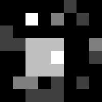
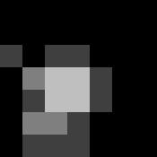
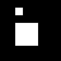
Original image:
The values in these images are 0, 1, 2, 3, and 4. Values of X.5 and below were rounded down to the nearest integer, and above X.5 were rounded up. Values beyond the range were clipped. Another option would be to scale the values so that there are no values beyond the range of available pixel values.
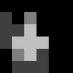
Averaging (lowpass) filter with 2x2 mask:
The mask used was:
| 1/4 | 1/4 |
| 1/4 | 1/4 |
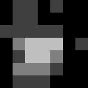
This filter will smooth out sharp transitions (high frequencies), so it can get rid of sharp noise, but will also get rid of sharp aspects in the image that you may want to keep.
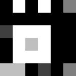
Averaging (lowpass) filter with 3x3 mask:
The mask used was:
| 1/9 | 1/9 | 1/9 |
| 1/9 | 1/9 | 1/9 |
| 1/9 | 1/9 | 1/9 |
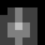
Compared with the 2x2 averaging filter, this 3x3 filter will result in an even smoother image, potentially getting rid of more sharp noise but also eliminating more image details.
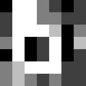
Weighted average 3x3:
The mask used is:
| 1/18 | 1/18 | 1/18 |
| 1/18 | 10/18 | 1/18 |
| 1/18 | 1/18 | 1/18 |
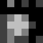
This filter shows some of the same results as the averaging filters, such as reduced high frequency components, but since the original pixel value is heavily weighted, the resulting image preserves more of the original image. The result is less blending, even with the 3x3 (which is large for an 8x8 image), yet also less reduction of sharp noise.
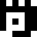
Median filter 2x2:
Compared with the 2x2 averaging filter, the median preserves more of the edges and contour of the main object in the image while getting rid of even more of the very sharp peripheral noise.
Median filter 3x3:
Compared with the 2x2 median filter, this 3x3 filter will smooth a bit more, yet still without the level of edge-mushing that we see with a 3x3 averaging filter.
High pass (sharpening) filter:
The mask used is:
| -1/9 | -1/9 | -1/9 |
| -1/9 | 8/9 | -1/9 |
| -1/9 | -1/9 | -1/9 |

This filter does the opposite of our example of lowpass filters (averaging) above. Note that it highlights the sharp transitions of the edges of the main object as well as the points of surrounding noise.
High boost filter:
The mask used is:
| -1/9 | -1/9 | -1/9 |
| -1/9 | 17/9 | -1/9 |
| -1/9 | -1/9 | -1/9 |
The high boost can be thought of as subtracting a lowpass component from the original or else as adding a highpass component to the original. The effect is accentuated sharp transitions (such as edges and small areas of noise) like the high pass filter but with more of the original image left in. So instead of having a resulting image of just the outline of your objects, you have an image of your objects with bright outlines.
Roberts (gradient/derivative/difference) filter:
Two masks were used on this image. The final pixel value was the sum of the absolute values of the two masks. The two masks were:
| 1 | 0 | 0 | 1 | |
| 0 | -1 | -1 | 0 |
There are many ways of implementing the gradient effect. One way is with this Roberts filter, which sums the magnitude of the differences across the target pixel diagonally. Note that the gradient effect sharpens the image (the outline of the main object is (nicely) accented, and also the background has many new (perhaps not so nice) sharp transitions.)
Threshold:
Values >= 3 were set to 4. Values < 3 were set to 0.
This threshold value happened to be appropriate for our main square in our original image, and the square was isolated very well. However, so was a point of noise, and we aren't always so lucky with the values in the main object. Thresholding can be a very powerful post-filtering technique to highlight aspects found with other filters.
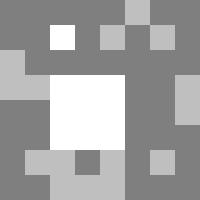
Thresholding with a local average:
First a 3x3 average was taken. If the pixel value was greater than that average, set the pixel to 4. Otherwise, set it to 0.
This filter is helpful when there is a systematic change in overall intensities in an image. Note that it highlights the outline of the main object. However, there are several point noise spots that are also highlighted. Some ways to reduce these spots are to take a larger area for the initial average and to use a threshold value that is a little above the actual average to account for small noise variations in constant areas of the image.
Connectivity:
This is one of many definitions of connectivity. Start with the center pixel and set it to 4. The look at its 4-neighbors. (4-neighbors are the 4 neighboring pixels which are not diagonal to the current pixel.) If a 4-neighbor value is within 1 of the current value pixel, that pixel is counted as "in" and is set to 4.

Given a good starting point in a desired area, this concept can be used to aid in segmentation of images.
Histogram equalization.
The pixel values that were originally value k are set to the value: sum(from 0 to k) of (n*V)/N, where n = unnormalized height of histogram bin k, N = total number of pixels, and V = highest pixel value. So for example, all the pixels that used to have value 2 in the original image would now be: (39*4)/64 + (11*4)/64 = 3.1250 rounded to 3. (Since there are 39 pixels with value 0 in the original image, 11 with value 1, 64 total pixels, and a high possible value of 4.)
Note that the resulting histogram is not exactly flat. This is because we cannot separate values that are in the same histogram bin. That is, we can't assign half of the 0-pixels to be changed to 1 and the other half to be changed to 2, because how could we possibly make the decisions as to which pixels get to become which number. In the more general technique called histogram specification, you can choose other shapes that you mold the histogram to look like.
Point processing
Pixel map used:
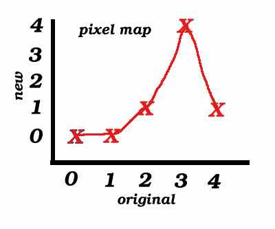
This is similar to histogram equalization in that it assigns new values to pixels from a lookup table, but it is more general than histogram equalization. Here we were able to specify any pixel mapping we wanted. Note in particular that the map is not monotonically increasing as it must be with most histogram manipulation. With a monotonically increasing function, the order of the intensity values will be preserved. That is, a pixel that was originally darker than another pixel will never end up brighter than that second pixel. In this particular mapping, the brightest pixels end up quite dark. Our processing isolated the main object while minimizing surrounding noise quite well, but note that our choice of a pixel map was based on specialized knowledge of the characteristics of our image (for instance, that our main object and only our main object has mainly value 3), knowledge that we often don't have in a real imaging situation.