Name 1:
Login: ee16a-
Name 2:
Login: ee16a-
Introduction
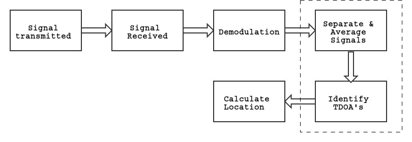
Last week we learned to use a powerful tool, cross-correlation, to extract information from the received signal. In this week's lab, you will continue to process the information you have extracted last week, and do some locationing! Just like last week's lab you will focus first on implementing and testing, and it may be confusing. Feel free to ask when you are stuck (you are not alone!), and use plots and visualizations to help yourself understand the materials!
%pylab inline
from __future__ import division
import random
import math

# Importing helper functions
%run wk2_code/virtual.py
%run wk2_code/signals.py
%run wk2_code/demod.py
Task 0: Importing Week 1 Code
This lab will require you to use the three functions you implemented last week.
**
Copy the cross_correlation and identify_peak functions into the cell below.
**
Alternatively if you have them saved in a .py file you can replace the cell below with the command:
%run [path_to_your_file].py.
This is the same syntax used to import the helper functions above.
# Copy the functions from week 1 below
def cross_correlation(signal1, signal2):
    """Compute the cross_correlation of two given signals
    Args:
    signal1 (np.array): input signal 1
    signal2 (np.array): input signal 2

    Returns:
    cross_correlation (np.array): cross-correlation of signal1 and signal2

    >>> cross_correlation([0, 1, 2, 3, 3, 2, 1, 0], [0, 2, 3, 0])
    [0, 0, 3, 8, 13, 15, 12, 7, 2, 0, 0]
    >>> cross_correlation([0, 2, 3, 0], [0, 1, 2, 3, 3, 2, 1, 0])
    [0, 0, 2, 7, 12, 15, 13, 8, 3, 0, 0]
    """
    # YOUR CODE HERE #

def identify_peak(signal):
    """Returns the index of the peak of the given signal.
    Args:
    signal (np.array): input signal

    Returns:
    index (int): index of the peak

    >>> identify_peak([1, 2, 5, 7, 12, 4, 1, 0])
    4
    >>> identify_peak([1, 2, 2, 199, 23, 1])
    3
    """
    # YOUR CODE HERE #
Task 1: Separating Beacons
Recall from the last week's lab although we only have a single microphone receiving signals from multiple beacons, we can use cross-correlation to determine the time (in samples) that each of the signals arrived. We call this process separating signals.
Complete the separate signal function.
# A list of simulated beacons has been imported already. Any code requiring the original beacons can just use this.
beacon
def separate_signal(raw_signal):
    """Separate the beacons by computing the cross correlation of the raw demodulated signal
    with the known beacon signals.

    Args:
    raw_signal (np.array): raw demodulated signal from the microphone composed of multiple beacon signals

    Returns (list): each entry should be the cross-correlation of the signal with one beacon
    """
    # YOUR CODE HERE #
Before we move on to converting these time differences into locations, we first need to consider several potential issues with our locationing system.
- Our beacons are being played repeatedly at a fixed rate, however we don't know when in the sequence of beacons we started recording. For example, if we record exactly the number of samples of a beacon, we may have began recording after some of the beacon signals reached the microphone.
- The microphone uses a buffer to allow it to output data to the computer the appropriate rate when the recording function is called. When recording samples are first saved to this buffer, and unfortunately when we first start recording we don't know what it contains. This is why you may have only seen your signal "start" at a certian time as shown below.
- You may have noticed last week that the height of the peaks in your final output was dependent on the volume of the speakers. Just like all of the other systems, the output will be affected by noise which in this case is literally other sounds in the room.
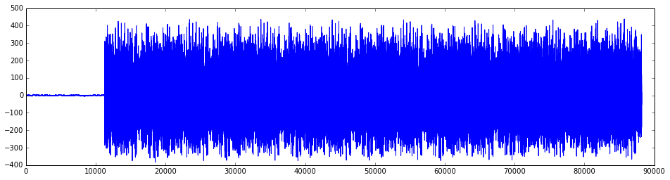 The low amplitude values before sample 10,000 correspond to values read from the buffer prior to recording the real signal.
The beacon signals repeat every 52 ms, and we record for approximately 2.5 s. Because of this we are recording the same beacon signals multiple times, and assuming our object isn't moving we only need one set of measurements to determine the time differences between them.
How can we use our full recorded signal to solve the problems explained above and make our system more robust?
Hint: In week 3 of the imaging module we explored a method of using multiple measurements to produce a higher quality image.
We have implemented a function that makes this improvement below. The mathematical operation it performs should be obvious by now, but make sure you can explain what each line of code is doing for checkoff.
def average_signal(separated):
    beacon_length = len(beacon0)
    num_repeat = len(separated) // beacon_length
    averaged = np.mean(np.abs(separated[0 : num_repeat * beacon_length]).reshape((num_repeat, beacon_length)), 0)
    return averaged

def signal_generator(x, y, noise=0):
    raw_signal = add_random_noise(simulate_by_location(x, y), noise)
    return demodulate_signal(raw_signal)
Run the code below to plot how the quality of the signal improves after running this function.
Note: Each of these blocks deals with >100k samples, so they may take some time to run.
test_signal = signal_generator(1.2, 3.4, noise=25)
sig = separate_signal(test_signal)
plt.figure(figsize=(16,4))
plt.plot(np.abs(sig[1]))
plt.title('2.5 sec Recording of Beacon 1 After Separation\n(No Averaging)')
plt.show()
avg = [average_signal(s) for s in sig]
plt.figure(figsize=(16,4))
plt.plot(avg[1])
plt.title('Averaged Output for Beacon 1')
plt.show()
What is the effect of averaging? Why would this be useful?
Task 2a: Computing Distances
We can now determine the time each signal arrived with respect to the first sample of the recording. Unfortunately, this time in samples has no direct relationship to physical distances and as discussed above our recordings start at arbitrary times with respect to the beacons. We can however compute times relative to a particular beacon.
For example, if our cross-correlation tells us that beacon1 arrives at $t_1 = 1120$ and beacon2 arrives at $t_2 = 1420$ we can see that beacon2 arrives $300$ samples after beacon1.
We call the relative time of arrival in samples offsets and define the offset with respect to beacon0.
According to our definition above what is the offset of beacon0?
If beacon2 arrives 450 samples later than beacon0, what is the time difference of arrival (in seconds) given that our sampling rate is $f_s=44100$ Hz?
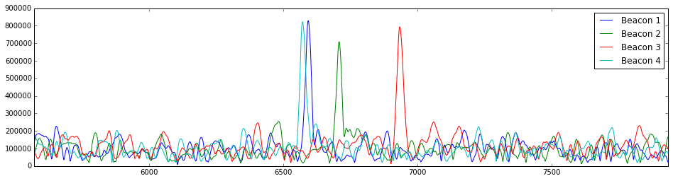
Run the code below to plot the separated signals. Can you estimate the offset for each signal relative to beacon 0?
# Simulate the demodulated microhpone output
test_signal = signal_generator(1.4, 3.22)

# Separate the beacon signals
separated = separate_signal(test_signal)

# Perform our averaging function
avg = [average_signal(s) for s in separated]

# Plot the averaged output for each beacon
plt.figure(figsize=(16,4))
for i in range(len(avg)):
    plt.plot(avg[i], label="{0}".format(i))
plt.title("Separated and Averaged Signals")
plt.legend()
plt.show()

# Plot the averaged output for each beacon centered about beacon0
plt.figure(figsize=(16,4))
peak = identify_peak(avg[0])
for i in range(len(avg)):
    plt.plot(np.roll(avg[i], len(avg[0]) // 2 - peak), label="{0}".format(i))
plt.title("Shifted")
plt.legend()
plt.show()
Note that sometimes a beacon can arrive earlier than the first signal. Our plot above shows these beacons are at the very end. More intuitively, these beacons have a negative offset and should arrive before beacon0. You can think of this as the plot being a defined number of samples and the end wrapping around to represent negative values.
We have provided you code to center the received signal about beacon0 at sample 0.
Complete the function below which returns offsets in samples given a list of input signals.
def identify_offsets(averaged):
    """ Identify the difference in samples between the samples.
    The peaks of the signals are shifted to the center.

    Args:
    averaged (list): a python list in which each entry is a numpy array (e.g. output of average_signal)

    Returns: (list) a list corresponding to the offset of each signal in the input
    """
    # Reshaping (shifting) the input so that all of our peaks are centered about the peak of beacon0
    peak = identify_peak(averaged[0])
    shifted = [np.roll(avg, len(averaged[0]) // 2 - peak) for avg in averaged]
    ##### DO NOT CHANGE THE CODE ABOVE THIS LINE ####

    # shifted represents all of the signals shifted so that they are centered about the peak of beacon0
    # use shifted to determine the offsets
    # consider what the offset for beacon0 should be
    # YOUR CODE HERE #
We now need to convert the offsets we have computed in samples to the time difference of arrivals (TDOAs) we will use to determine locations. to TDOA's before we can use them to do locationing. Implement a function offset_to_time, which takes a list of offsets, and sampling frequency and returns a list of TDOA's.
Given that our microphones sample at a rate of $f_s=44100$ Hz, complete the function offset_to_time below which takes a list of offsets (for example the output of identify_offsets), and a sampling frequency and returns a list of TDOA's.
Hint: What is the relation between sampling frequency, number of samples, and time?
def offset_to_time(offsets, sampling_freq):
    """ Convert a list of offsets to a list of TDOA's

    Args:
    offsets (list): list of offests in samples
    sampling_freq (int): sampling frequency in Hz

    Returns: (list) a list of TDOAs corresponding to the input offsets
    """
    # YOUR CODE HERE #
Task 2b: Combining Functions
We now have a variety of helper functions to perform each step of the calculations required to go from our microphone signal to a list TDOAs.
Implement a function that will take in the recorded microphone signal and output the offset in samples.
def signal_to_offsets(raw_signal):
    """ Compute a list of offsets from the microphone to each speaker.

    Args:
    raw_signal (np.array): raw demodulated signal from the microphone (e.g. no separation, averaging, etc).

    Returns (list): offset for each beacon (beacon0, beacon1, etc). in samples
    """
    # YOUR CODE HERE #
We now know the time differences relative to a single beacon, so given a reference time for beacon0 we can determine the total time for the sound wave to travel the distance from the speakers to our microphone. Knowing that the speed of sound is 340 m/s, we can compute the distance from the microphone to each speaker, and use simple geometry to locate ourselves! This is exactly what the GPS is doing, except with electromagnetic waves rather than sound waves.
Implement a function, signal_to_distances, which takes a recorded signal and the time of arrival of the first beacon signal, and returns a list of the distance from the microphone to each speaker.
Hint: You may wish to take advantage of a function that computes the offsets given the raw demodulated microphone signal.
def signal_to_distances(raw_signal, t0):
    """ Returns a list of distancs from the microphone to each speaker.

    Args:
    signal (np.array): recorded signal from the microphone
    t0 (float): reference time for beacon0 in seconds

    Returns (list): distances to each of the speakers (beacon0, beacon1, etc). in meters
    """
    # YOUR CODE HERE #
After computing the distances from each speaker, we can use the formula for distance $d = \sqrt{(x-x_{speaker})^2 + (y-y_{speaker})^2}$ to construct a system of equations and solve for our exact location! Rather than solving for our exact coordinates, we will visualize our position with respect to the beacons on a graph.
Run the following block that uses your signal_to_distance function to simulate speakers located at (0, 0), (5, 0), (0, 5) on a 2D plane and a microphone located at (1.2, 3.6).
# Assume the time of arrival of the first beacon is 0.011151468430462413.
received_signal = get_signal_virtual(x=1.2, y=3.6)
demod = demodulate_signal(received_signal)
distances = signal_to_distances(demod, 0.011151468430462413)
distances = distances[:3]
print("The distances are: " + str(distances))

# Plot the speakers
plt.scatter([0, 5, 0], [0, 0, 5], marker='x', color='b', label='Speakers')
d0 = plt.Circle((0, 0), distances[0],facecolor='none', ec='r')
d1 = plt.Circle((5, 0), distances[1],facecolor='none', ec='g')
d2 = plt.Circle((0, 5), distances[2],facecolor='none', ec='c')
fig = plt.gcf()
fig.gca().add_artist(d0)
fig.gca().add_artist(d1)
fig.gca().add_artist(d2)
plt.xlim(-8, 8)
plt.ylim(-16/3, 16/3)
plt.legend()
plt.show()
What do you observe? What does each circle mean? What about their intersections?
Now let's explore how the number of speakers (beacon signals) affect our solution. First, let try the exact same code with one less beacon signal (so we only have two beacons and the time of arrival of the first one):
# Assume the time of arrival of the first beacon is 0.011151468430462413.
received_signal = get_signal_virtual(x=1.2, y=3.6)
demod = demodulate_signal(received_signal)
distances = signal_to_distances(demod, 0.011151468430462413)
distances = distances[:2]
print("The distances are: " + str(distances))

# Plot the speakers
plt.scatter([0, 5, 0], [0, 0, 5], marker='x', color='b', label='Speakers')
d0 = plt.Circle((0, 0), distances[0],facecolor='none', ec='r')
d1 = plt.Circle((5, 0), distances[1],facecolor='none', ec='g')
fig = plt.gcf()
fig.gca().add_artist(d0)
fig.gca().add_artist(d1)
plt.xlim(-6, 6)
plt.ylim(-4, 4)
plt.legend()
plt.show()
How many dimensions can we determine our position in? For our goal of a 2D locationing system what is the minimum number of beacons we will need?
Now let's do it with five beacons:
# Assume the time of arrival of the first beacon is 0.011151468430462413.
received_signal = get_signal_virtual(x=1.2, y=3.6)
demod = demodulate_signal(received_signal)
distances = signal_to_distances(demod, 0.011151468430462413)
distances = distances[:5]
print("The distances are: " + str(distances))

# Plot the speakers
plt.scatter([0, 5, 0, 5, 0], [0, 0, 5, 5, 2.5], marker='x', color='b', label='Speakers')
d0 = plt.Circle((0, 0), distances[0],facecolor='none', ec='r')
d1 = plt.Circle((5, 0), distances[1],facecolor='none', ec='g')
d2 = plt.Circle((0, 5), distances[2],facecolor='none', ec='c')
d3 = plt.Circle((5, 5), distances[3],facecolor='none', ec='y')
d4 = plt.Circle((0, 2.5), distances[4],facecolor='none', ec='m')

fig = plt.gcf()
fig.gca().add_artist(d0)
fig.gca().add_artist(d1)
fig.gca().add_artist(d2)
fig.gca().add_artist(d3)
fig.gca().add_artist(d4)
plt.xlim(-8, 8)
plt.ylim(-16/3, 16/3)
plt.legend()
plt.show()
We know we need a minimum number of beacons to find our location uniquely in a 2D space. How could additional beacons be useful?
Run the following tests and make sure that all 4 are passing before moving on to the microphone section.
# Virtual Test

# Utility Functions
def list_float_eq(lst1, lst2):
    if len(lst1) != len(lst2): return False
    for i in range(len(lst1)):
        if abs(lst1[i] - lst2[i]) >= 0.00001: return False
    return True

def list_sim(lst1, lst2):
    if len(lst1) != len(lst2): return False
    for i in range(len(lst1)):
        if abs(lst1[i] - lst2[i]) >= 3: return False
    return True

test_num = 0

# 1. Identify offsets - 1
test_num += 1
test_signal = get_signal_virtual(offsets = [0, 254, 114, 22, 153, 625])
demod = demodulate_signal(test_signal)
sig = separate_signal(demod)
avg = [average_signal(s) for s in sig]
offsets = identify_offsets(avg)
test = list_sim(offsets, [0, 254, 114, 22, 153, 625])
if not test:
    print("Test {0} Failed".format(test_num))
else: print("Test {0} Passed".format(test_num))

# 2. Identify offsets - 2
test_num += 1
test_signal = get_signal_virtual(offsets = [0, -254, 0, -21, 153, -625])
demod = demodulate_signal(test_signal)
sig = separate_signal(demod)
avg = [average_signal(s) for s in sig]
offsets = identify_offsets(avg)
test = list_sim(offsets, [0, -254, 0, -21, 153, -625])
if not test:
    print("Test {0} Failed".format(test_num))
else: print("Test {0} Passed".format(test_num))

# 3. Offsets to TDOA
test_num += 1
test = list_float_eq(offset_to_time([0, -254, 0, -21, 153, -625], 44100), [0.0, -0.005759637188208617, 0.0, -0.0004761904761904762, 0.0034693877551020408, -0.01417233560090703])
if not test:
    print("Test {0} Failed".format(test_num))
else: print("Test {0} Passed".format(test_num))

# 4. Signal to distances
test_num += 1
dist = signal_to_distances(demodulate_signal(get_signal_virtual(x=1.765, y=2.683)), 0.009437530220245524)
test = list_float_eq(dist, [3.2114971586473495, 4.199186954565717, 2.9182767504840843, 3.975413485177962, 1.776260423953472, 2.7870991994636762])
if not test:
    print("Test {0} Failed".format(test_num))
else: print("Test {0} Passed".format(test_num))
We can now locate ourselves if we know the time of arrival of the first beacon. How can we do it without knowing any time of arrival? In next week's lab, we will find a way to do the locationing using only time difference of arrival (TDOA's)!
Post Lab Homework: Copy signal_to_offsets, and all functions it depends on, into lab2.py. You will need to paste them to the next week's notebook just like this week.
Testing Area for Week Two
We have several tests written for you. Before you test on the microphone, you should make sure that you code passes these tests.
%run wk2_code/rec.py

def get_signal():
    """Get the signal from the microphone"""
    return mic.new_data()
Play offset250_540-321.wav in the lab folder and use your microphone to record it (by running the cell below - you may want to run it for several times when the wav file is playing to clear the buffer.
received_signal = get_signal()
Again, plot the signal to make sure it is properly recorded before you use it to test your code.
plt.figure(figsize=(16,4))
plt.plot(received_signal)
plt.show()
# Test your code:
offsets = signal_to_offsets(demodulate_signal(received_signal))
print("Expected: " + str([0, 250, 540, -321]))
print("Got: " + str(offsets[:4]))