 Programming Project #5 (proj5)
CS180: Intro to Computer Vision and Computational Photography
Programming Project #5 (proj5)From the lecture we know that we can use a Neural Radiance Field (NeRF) (\(F: \{x, y, z, \theta, \phi\} \rightarrow \{r, g, b, \sigma\}\)) to represent a 3D space. But before jumping into 3D, let's first get familar with NeRF (and PyTorch) using a 2D example. In fact, since there is no concept of radiance in 2D, the Neural Radiance Field falls back to just a Neural Field (\(F: \{u, v\} \rightarrow \{r, g, b\}\)) in 2D, in which \(\{u, v\}\) is the pixel coordinate. In this section, we will create a neural field that can represent a 2D image and optimize that neural field to fit this image. You can start from this image, but feel free to try out any other images.
[Impl: Network] You would need to create an Multilayer Perceptron (MLP) network with Sinusoidal Positional Encoding (PE) that takes in the 2-dim pixel coordinates, and output the 3-dim pixel colors.

[Impl: Dataloader] If the image is with high resolution, it might be not feasible train the network with the all the pixels in every iteration due to the GPU memory limit. So you need to implement a dataloader that randomly sample \(N\) pixels at every iteration for training. The dataloader is expected to return both the \(N\times2\) 2D coordinates and \(N\times3\) colors of the pixels, which will serve as the input to your network, and the supervision target, respectively (essentially you have a batch size of \(N\)). You would want to normalize both the coordinates (x = x / image_width, y = y / image_height) and the colors (rgbs = rgbs / 255.0) to make them within the range of [0, 1].
[Impl: Loss Function, Optimizer, and Metric] Now that you have the network (MLP) and the dataloader, you need to define the loss function and the optimizer before you can start training your network. You will use mean squared error loss (MSE) (torch.nn.MSELoss) between the predicted color and the groundtruth color. Train your network using Adam (torch.optim.Adam) with a learning rate of 1e-2. Run the training loop for 1000 to 3000 iterations with a batch size of 10k. For the metric, MSE is a good one but it is more common to use Peak signal-to-noise ratio (PSNR) when it comes to measuring the reconstruction quality of a image. If the image is normalized to [0, 1], you can use the following equation to compute PSNR from MSE: \[PSNR = 10 \cdot log_{10}\left(\frac{1}{MSE}\right)\]
[Impl: Hyperparameter Tuning] Try varying two of the hyperparameters (number of layers, channel size, max frequency \(L\) for the positional encoding, or learning rate) and show how it affects (or doesn't affect) the performance of your network.

[Deliverables] As a reference, the above images show the process of optimizing the network to fit on this image.
Now that we are familiar with using a neural field to represent a image, we can proceed to a more interesting task that using a neural radiance field to represent a 3D space, through inverse rendering from multi-view calibrated images. For this part we are going to use the Lego scene from the original NeRF paper, but with lower resolution images (200 x 200) and preprocessed cameras (downloaded from here). The following code can be used to parse the data. The figure on its right shows a plot of all the cameras, including training cameras in black, validation cameras in red, and test cameras in green.
data = np.load(f"lego_200x200.npz")

# Training images: [100, 200, 200, 3]
images_train = data["images_train"] / 255.0

# Cameras for the training images
# (camera-to-world transformation matrix): [100, 4, 4]
c2ws_train = data["c2ws_train"]

# Validation images:
images_val = data["images_val"] / 255.0

# Cameras for the validation images: [10, 4, 4]
# (camera-to-world transformation matrix): [10, 200, 200, 3]
c2ws_val = data["c2ws_val"]

# Test cameras for novel-view video rendering:
# (camera-to-world transformation matrix): [60, 4, 4]
c2ws_test = data["c2ws_test"]

# Camera focal length
focal = data["focal"]  # float

Camera to World Coordinate Conversion. The transformation between the world space \(\mathbf{X_w} = (x_w, y_w, z_w)\) and the
camera space \(\mathbf{X_c} = (x_c, y_c, z_c)\) can be defined as a rotation matrix \(\mathbf{R}_{3\times3}\) and a translation vector
\(\mathbf{t}\): \[\begin{align} \begin{bmatrix} x_c \\ y_c \\ z_c \\ 1 \end{bmatrix} = \begin{bmatrix} \mathbf{R}_{3\times3} &
\mathbf{t} \\ \mathbf{0}_{1\times3} & 1 \end{bmatrix} \begin{bmatrix} x_w \\ y_w \\ z_w \\ 1 \end{bmatrix} \end{align}\] in which
\(\begin{bmatrix} \mathbf{R}_{3\times3} & \mathbf{t} \\ \mathbf{0}_{1\times3} & 1 \end{bmatrix}\) is called world-to-camera
(w2c) transformation matrix, or extrinsic matrix. The inverse of it is called camera-to-world (c2w)
transformation matrix.
[Impl] In this session you would need to implement a function x_w = transform(c2w, x_c) that transform a point
from camera to the world space. You can verify your implementation by checking if the follow statement is always true:
x == transform(c2w.inv(), transform(c2w, x)). Note you might want your implementation to support batched coordinates for
later use. You can implement it with either numpy or torch.
Pixel to Camera Coordinate Conversion. Consider a pinhole camera with focal length \((f_x, f_y)\) and principal point \((o_x = \text{image_width} / 2, o_y = \text{image_height} / 2)\), it's intrinsic matrix \(\mathbf{K}\) is defined as: \[\begin{align} \mathbf{K} = \begin{bmatrix} f_x & 0 & o_x \\ 0 & f_y & o_y \\ 0 & 0 & 1 \end{bmatrix} \end{align}\] which can be used to project a 3D point \((x_c, y_c, z_c)\) in the camera coordinate system to a 2D location \((u, v)\) in pixel coordinate system : \[\begin{align} s \begin{bmatrix} u \\ v \\ 1 \end{bmatrix} = \mathbf{K} \begin{bmatrix} x_c \\ y_c \\ z_c \end{bmatrix} \end{align}\] in which \(s=z_c\) is the depth of this point along the optical axis.
[Impl] In this session you would need to implement a function that invert the aforementioned process, which transform a point
from the pixel coordinate system back to the camera coordinate system: x_c = pixel_to_camera(K, uv, s). Similar to the
previous session, you might also want your implementation here to support batched coordinates for later use. You can implement it with
either numpy or torch.
Pixel to Ray. A ray can be defined by an origin \(\mathbf{r}_o \in R^3\) vector and a direction \(\mathbf{r}_d \in R^3\) vector. So in the case of pinhole camera, we want to know the \(\{\mathbf{r}_o, \mathbf{r}_d\}\) for every pixel \((u, v)\). The origin \(\mathbf{r}_o\) of those rays are eazy to get because it is just the location of the cameras: \[\begin{align} \mathbf{r}_o = -\mathbf{R}_{3\times3}^{-1}\mathbf{t} \end{align}\] To calculate the ray direction for pixel \((u, v)\), we can simply choose a point along this ray with depth equals 1 (\(s=1\)) and find its coordinate in the world space \(\mathbf{X_w} = (x_w, y_w, z_w)\). Then the normalized ray direction can be computed by: \[\begin{align} \mathbf{r}_d = \frac{\mathbf{X_w} - \mathbf{r}_o}{||\mathbf{X_w} - \mathbf{r}_o||_2} \end{align}\]
[Impl] In this session you would need to implement this function that convert a pixel coordinate to a ray with origin and
noramlized direction: ray_o, ray_d = pixel_to_ray(K, c2w, uv). You might find your previously implemented functions
useful here. Similarly you might also want your implementation here to support batched coordinates.
[Impl: Sampling Rays from Images] In Part 1, we have done random sampling on a single image to get the pixel color and pixel coordinates. Here we can build on top of that, and with the camera intrinsics & extrinsics, we would be able to convert the pixel coordinates into ray origins and directions. Make sure to account for the offset from image coordinate to pixel center (this can be done simply by adding .5 to your UV pixel coordinate grid)! Since we have multiple images now, we have two options of sampling rays. Say we want to sample N rays at every training iteration, option 1 is to first sample M images, and then sample N // M rays from every image. The other option is to flatten all pixels from all images and do a global sampling once to get N rays from all images. You can choose which ever way do ray sampling.
[Impl: Sampling Points along Rays.] After having rays, we also need to discritize each ray into samples that live in the 3D
space. The simplist way is to uniformly create some samples along the ray (t = np.linspace(near, far, n_samples)). For
the lego scene that we have, we can set near=2.0 and far=6.0. The actually 3D corrdinates can be accquired
by \(\mathbf{x} = \mathbf{R}_o + \mathbf{R}_d * t\). However this would lead to a fixed set of 3D points, which could potentially lead
to overfitting when we train the NeRF later on. On top of this, we want to introduce some small perturbation to the points
only during training, so that every location along the ray would be touched upon during training. this can be achieved by
something like t = t + (np.random.rand(t.shape) * t_width) where t is set to be the start of each interval. We recommend
to set n_samples to 32 or 64 in this project.
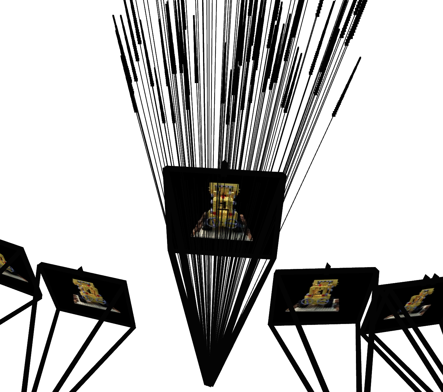
Similar to Part 1, you would need to write a dataloader that randomly sample pixels from multiview images. What is different with Part 1, is that now you need to convert the pixel coordinates into rays in your dataloader, and return ray origin, ray direction and pixel colors from your dataloader. To verify if you have by far implement everything correctly, we here provide some visualization code to plot the cameras, rays, and samples in 3D. We additionally recommend you try this code with rays sampled only from one camera so you can make sure that all the rays stay within the camera frustum and eliminating the possibility of other smaller harder to catch bugs.
import viser, time  # pip install viser
import numpy as np

# --- You Need to Implement These ------
dataset = RaysData(images_train, K, c2ws_train)
rays_o, rays_d, pixels = dataset.sample_rays(100) # Should expect (B, 3)
points = sample_along_rays(rays_o, rays_d, perturb=True)
H, W = images_train.shape[1:3]
# ---------------------------------------

server = viser.ViserServer(share=True)
for i, (image, c2w) in enumerate(zip(images_train, c2ws_train)):
    server.add_camera_frustum(
        f"/cameras/{i}",
        fov=2 * np.arctan2(H / 2, K[0, 0]),
        aspect=W / H,
        scale=0.15,
        wxyz=viser.transforms.SO3.from_matrix(c2w[:3, :3]).wxyz,
        position=c2w[:3, 3],
        image=image
    )
for i, (o, d) in enumerate(zip(rays_o, rays_d)):
    server.add_spline_catmull_rom(
        f"/rays/{i}", positions=np.stack((o, o + d * 6.0)),
    )
server.add_point_cloud(
    f"/samples",
    colors=np.zeros_like(points).reshape(-1, 3),
    points=points.reshape(-1, 3),
    point_size=0.02,
)
time.sleep(1000)
# Visualize Cameras, Rays and Samples
import viser, time
import numpy as np

# --- You Need to Implement These ------
dataset = RaysData(images_train, K, c2ws_train)

# This will check that your uvs aren't flipped
uvs_start = 0
uvs_end = 40_000
sample_uvs = dataset.uvs[uvs_start:uvs_end] # These are integer coordinates of widths / heights (xy not yx) of all the pixels in an image
# uvs are array of xy coordinates, so we need to index into the 0th image tensor with [0, height, width], so we need to index with uv[:,1] and then uv[:,0]
assert np.all(images_train[0, sample_uvs[:,1], sample_uvs[:,0]] == dataset.pixels[uvs_start:uvs_end])

# # Uncoment this to display random rays from the first image
# indices = np.random.randint(low=0, high=40_000, size=100)

# # Uncomment this to display random rays from the top left corner of the image
# indices_x = np.random.randint(low=100, high=200, size=100)
# indices_y = np.random.randint(low=0, high=100, size=100)
# indices = indices_x + (indices_y * 200)

data = {"rays_o": dataset.rays_o[indices], "rays_d": dataset.rays_d[indices]}
points = sample_along_rays(data["rays_o"], data["rays_d"], random=True)
# ---------------------------------------

server = viser.ViserServer(share=True)
for i, (image, c2w) in enumerate(zip(images_train, c2ws_train)):
  server.add_camera_frustum(
    f"/cameras/{i}",
    fov=2 * np.arctan2(H / 2, K[0, 0]),
    aspect=W / H,
    scale=0.15,
    wxyz=viser.transforms.SO3.from_matrix(c2w[:3, :3]).wxyz,
    position=c2w[:3, 3],
    image=image
  )
for i, (o, d) in enumerate(zip(data["rays_o"], data["rays_d"])):
  positions = np.stack((o, o + d * 6.0))
  server.add_spline_catmull_rom(
      f"/rays/{i}", positions=positions,
  )
server.add_point_cloud(
    f"/samples",
    colors=np.zeros_like(points).reshape(-1, 3),
    points=points.reshape(-1, 3),
    point_size=0.03,
)
time.sleep(1000)

[Impl: Network] After having samples in 3D, we want to use the network to predict the density and color for those samples in 3D. So you would create a MLP that is similar to Part 1, but with three changes:
Below is a structure of the network that you can start with:

The core volume rendering equation is as follows: \[\begin{align} C(\mathbf{r})=\int_{t_n}^{t_f} T(t) \sigma(\mathbf{r}(t)) \mathbf{c}(\mathbf{r}(t), \mathbf{d}) d t, \text { where } T(t)=\exp \left(-\int_{t_n}^t \sigma(\mathbf{r}(s)) d s\right) \end{align}\]
This fundamentally means that at every small step \(dt\) along the ray, we add the contribution of that small interval \([t, t + dt]\) to that final color, and we do the infinitely many additions if these infintesimally small intervals with an integral.
The discrete approximation (thus tractable to compute) of this equation can be stated as the following: \[\begin{align} \hat{C}(\mathbf{r})=\sum_{i=1}^N T_i\left(1-\exp \left(-\sigma_i \delta_i\right)\right) \mathbf{c}_i, \text { where } T_i=\exp \left(-\sum_{j=1}^{i-1} \sigma_j \delta_j\right) \end{align}\] where \(\textbf{c}_i\) is the color obtained from our network at sample location \(i\), \(T_i\) is the probability of a ray not terminating before sample location \(i\), and \(1 - e^{-\sigma_i \delta_i}\) is the probability of terminating at sample location \(i\).
If your volume rendering works, the following snippet of code should pass the assert statement:
import torch
torch.manual_seed(42)
sigmas = torch.rand((10, 64, 1))
rgbs = torch.rand((10, 64, 3))
step_size = (6.0 - 2.0) / 64
rendered_colors = volrend(sigmas, rgbs, step_size)

correct = torch.tensor([
    [0.5006, 0.3728, 0.4728],
    [0.4322, 0.3559, 0.4134],
    [0.4027, 0.4394, 0.4610],
    [0.4514, 0.3829, 0.4196],
    [0.4002, 0.4599, 0.4103],
    [0.4471, 0.4044, 0.4069],
    [0.4285, 0.4072, 0.3777],
    [0.4152, 0.4190, 0.4361],
    [0.4051, 0.3651, 0.3969],
    [0.3253, 0.3587, 0.4215]
  ])
assert torch.allclose(rendered_colors, correct, rtol=1e-4, atol=1e-4)
[Impl] Here you will implement the volume rendering equation for a batch of samples along a ray. This rendered color is what we will compare with our posed images in order to train our network. You would need to implement this part in torch instead of numpy because we need the loss to be able to backpropagate through this part. A hint is that you may find torch.cumsum or torch.cumprod useful here.
[Deliverables] As a reference, the images below show the process of optimizing the network to fit on our lego multi-view images from a novel view. The staff solution reaches above 23 PSNR with 1000 gradient steps and a batchsize of 10K rays per gradent step. The staff solution uses an Adam optimizer with a learning rate of 5e-4. For guaranteed full credit, achieve 23 PSNR for any number of iterations.

c2ws_test in the npz file). You should be
get a video like this (left is 10 after minutes training, right is 2.5 hrs training):