Project 5: Machine Learning
In this project you will build a neural network to classify digits, and more!
Introduction
This project will be an introduction to machine learning.
The code for this project contains the following files, available as a zip archive.
| Files you'll edit: | |||
models.py |
Perceptron and neural network models for a variety of applications | qLearningAgents.py |
Code for RL agents. |
| Files you should read but NOT edit: | |||
nn.py |
Neural network mini-library | ||
| Files you will not edit: | |||
autograder.py |
Project autograder | ||
backend.py |
Backend code for various machine learning tasks | ||
data |
Datasets for digit classification and language identification | ||
submission_autograder.py |
Submission autograder (generates tokens for submission) | ||
Files to Edit and Submit: You will fill in portions of models.py during the assignment. Please do not change the other files in this distribution.
Note: You only need to submit machinelearning.token, generated by running submission_autograder.py. It contains the evaluation results from your local autograder, and a copy of all your code. You do not need to submit any other files. See Submission for details.
Evaluation: Your code will be autograded for technical correctness. Please do not change the names of any provided functions or classes within the code, or you will wreak havoc on the autograder. However, the correctness of your implementation – not the autograder’s judgements – will be the final judge of your score. If necessary, we will review and grade assignments individually to ensure that you receive due credit for your work.
Academic Dishonesty: We will be checking your code against other submissions in the class for logical redundancy. If you copy someone else’s code and submit it with minor changes, we will know. These cheat detectors are quite hard to fool, so please don’t try. We trust you all to submit your own work only; please don’t let us down. If you do, we will pursue the strongest consequences available to us.
Proper Dataset Use: Part of your score for this project will depend on how well the models you train perform on the test set included with the autograder. We do not provide any APIs for you to access the test set directly. Any attempts to bypass this separation or to use the testing data during training will be considered cheating.
Getting Help: You are not alone! If you find yourself stuck on something, contact the course staff for help. Office hours, section, and the discussion forum are there for your support; please use them. If you can’t make our office hours, let us know and we will schedule more. We want these projects to be rewarding and instructional, not frustrating and demoralizing. But, we don’t know when or how to help unless you ask.
Discussion: Please be careful not to post spoilers.
Installation
For this project, you will need to install the following two libraries:
- numpy, which provides support for large multi-dimensional arrays - installation instructions
- matplotlib, a 2D plotting library - installation instructions
If you have a conda environment, you can install both packages on the command line by running:
conda activate [your environment name]
pip install numpy
pip install matplotlib
You will not be using these libraries directly, but they are required in order to run the provided code and autograder.
To test that everything has been installed, run:
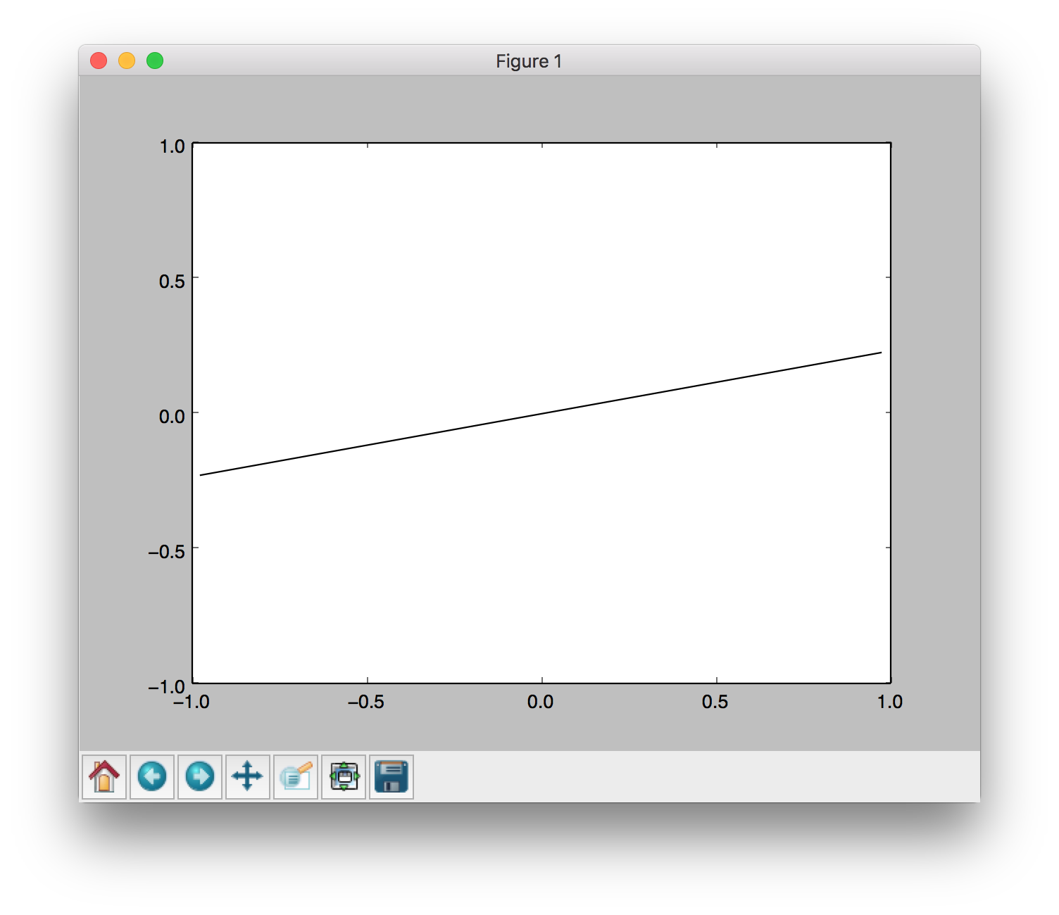
python autograder.py --check-dependencies
If numpy and matplotlib are installed correctly, you should see a window pop up where a line segment spins in a circle:
Provided Code (Part I)
For this project, you have been provided with a neural network mini-library (nn.py) and a collection of datasets (backend.py).
The library in nn.py defines a collection of node objects. Each node represents a real number or a matrix of real numbers. Operations on node objects are optimized to work faster than using Python’s built-in types (such as lists).
Here are a few of the provided node types:
nn.Constantrepresents a matrix (2D array) of floating point numbers. It is typically used to represent input features or target outputs/labels. Instances of this type will be provided to you by other functions in the API; you will not need to construct them directly.nn.Parameterrepresents a trainable parameter of a perceptron or neural network.nn.DotProductcomputes a dot product between its inputs.
Additional provided functions:
nn.as_scalarcan extract a Python floating-point number from a node.
When training a perceptron or neural network, you will be passed a dataset object. You can retrieve batches of training examples by calling dataset.iterate_once(batch_size):
for x, y in dataset.iterate_once(batch_size):
...
For example, let’s extract a batch of size 1 (i.e., a single training example) from the perceptron training data:
>>> batch_size = 1
>>> for x, y in dataset.iterate_once(batch_size):
...     print(x)
...     print(y)
...     break
...
<Constant shape=1x3 at 0x11a8856a0>
<Constant shape=1x1 at 0x11a89efd0>
The input features x and the correct label y are provided in the form of nn.Constant nodes. The shape of x will be batch_size x num_features, and the shape of y is batch_size x num_outputs. Here is an example of computing a dot product of x with itself, first as a node and then as a Python number.
>>> nn.DotProduct(x, x)
<DotProduct shape=1x1 at 0x11a89edd8>
>>> nn.as_scalar(nn.DotProduct(x, x))
1.9756581717465536
Question 1 (6 points): Perceptron
Before starting this part, be sure you have numpy and matplotlib installed!
In this part, you will implement a binary perceptron. Your task will be to complete the implementation of the PerceptronModel class in models.py.
For the perceptron, the output labels will be either \(1\) or \(-1\), meaning that data points (x, y) from the dataset will have y be a nn.Constant node that contains either \(1\) or \(-1\) as its entries.
We have already initialized the perceptron weights self.w to be a \(1 \times \text{dimensions}\) parameter node. The provided code will include a bias feature inside x when needed, so you will not need a separate parameter for the bias.
Your tasks are to:
- Implement the
run(self, x)method. This should compute the dot product of the stored weight vector and the given input, returning annn.DotProductobject. - Implement
get_prediction(self, x), which should return \(1\) if the dot product is non-negative or \(-1\) otherwise. You should usenn.as_scalarto convert a scalarNodeinto a Python floating-point number. - Write the
train(self)method. This should repeatedly loop over the data set and make updates on examples that are misclassified. Use theupdatemethod of thenn.Parameterclass to update the weights. When an entire pass over the data set is completed without making any mistakes, 100% training accuracy has been achieved, and training can terminate.
In this project, the only way to change the value of a parameter is by calling parameter.update(direction, multiplier), which will perform the update to the weights: \[\text{weights} \gets \text{weights} + \text{direction} \cdot \text{multiplier} \] The direction argument is a Node with the same shape as the parameter, and the multiplier argument is a Python scalar.
To test your implementation, run the autograder:
python autograder.py -q q1
Note: the autograder should take at most 20 seconds or so to run for a correct implementation. If the autograder is taking forever to run, your code probably has a bug.
Neural Network Tips
In the remaining parts of the project, you will implement the following models:
Building Neural Nets
Throughout the applications portion of the project, you’ll use the framework provided in nn.py to create neural networks to solve a variety of machine learning problems. A simple neural network has layers, where each layer performs a linear operation (just like perceptron). Layers are separated by a non-linearity, which allows the network to approximate general functions. We’ll use the ReLU operation for our non-linearity, defined as \(relu(x) = \max(x, 0)\). For example, a simple two-layer neural network for mapping an input row vector \(\mathbf{x}\) to an output vector \(\mathbf{f}(\mathbf{x})\) would be given by the function:
\[\mathbf{f}(\mathbf{x}) = relu(\mathbf{x} \cdot \mathbf{W_1} + \mathbf{b_1}) \cdot \mathbf{W_2} + \mathbf{b}_2 \]
where we have parameter matrices \(\mathbf{W_1}\) and \(\mathbf{W_2}\) and parameter vectors \(\mathbf{b}_1\) and \(\mathbf{b}_2\) to learn during gradient descent. \(\mathbf{W_1}\) will be an \(i \times h\) matrix, where \(i\) is the dimension of our input vectors \(\mathbf{x}\), and \(h\) is the hidden layer size. \(\mathbf{b_1}\) will be a size \(h\) vector. We are free to choose any value we want for the hidden size (we will just need to make sure the dimensions of the other matrices and vectors agree so that we can perform the operations). Using a larger hidden size will usually make the network more powerful (able to fit more training data), but can make the network harder to train (since it adds more parameters to all the matrices and vectors we need to learn), or can lead to overfitting on the training data.
We can also create deeper networks by adding more layers, for example a three-layer net: \[ \mathbf{f}(\mathbf{x}) = relu(relu(\mathbf{x} \cdot \mathbf{W_1} + \mathbf{b_1}) \cdot \mathbf{W_2} + \mathbf{b}_2) \cdot \mathbf{W_3} + \mathbf{b_3} \]
Note on Batching
For efficiency, you will be required to process whole batches of data at once rather than a single example at a time. This means that instead of a single input row vector \(x\) with size \(i\), you will be presented with a batch of \(b\) inputs represented as a \(b \times i\) matrix \(X\). We provide an example for linear regression to demonstrate how a linear layer can be implemented in the batched setting.
Note on Randomness
The parameters of your neural network will be randomly initialized, and data in some tasks will be presented in shuffled order. Due to this randomness, it’s possible that you will still occasionally fail some tasks even with a strong architecture – this is the problem of local optima! This should happen very rarely, though – if when testing your code you fail the autograder twice in a row for a question, you should explore other architectures.
Practical tips
Designing neural nets can take some trial and error. Here are some tips to help you along the way:
- Be systematic. Keep a log of every architecture you’ve tried, what the hyperparameters (layer sizes, learning rate, etc.) were, and what the resulting performance was. As you try more things, you can start seeing patterns about which parameters matter. If you find a bug in your code, be sure to cross out past results that are invalid due to the bug.
- Start with a shallow network (just two layers, i.e. one non-linearity). Deeper networks have exponentially more hyperparameter combinations, and getting even a single one wrong can ruin your performance. Use the small network to find a good learning rate and layer size; afterwards you can consider adding more layers of similar size.
-
If your learning rate is wrong, none of your other hyperparameter choices matter. You can take a state-of-the-art model from a research paper, and change the learning rate such that it performs no better than random. A learning rate too low will result in the model learning too slowly, and a learning rate too high may cause loss to diverge to infinity. Begin by trying different learning rates while looking at how the loss decreases over time.
-
Smaller batches require lower learning rates. When experimenting with different batch sizes, be aware that the best learning rate may be different depending on the batch size.
- Refrain from making the network too wide (hidden layer sizes too large) If you keep making the network wider accuracy will gradually decline, and computation time will increase quadratically in the layer size – you’re likely to give up due to excessive slowness long before the accuracy falls too much. The full autograder for all parts of the project takes 2-12 minutes to run with staff solutions; if your code is taking much longer you should check it for efficiency.
- If your model is returning Infinity or NaN, your learning rate is probably too high for your current architecture.
-
Recommended values for your hyperparameters:
- Hidden layer sizes: between 10 and 400.
- Batch size: between 1 and the size of the dataset. For Q2 and Q3, we require that total size of the dataset be evenly divisible by the batch size.
- Learning rate: between 0.001 and 1.0.
- Number of hidden layers: between 1 and 3.
Provided Code (Part II)
Here is a full list of nodes available in nn.py. You will make use of these in the remaining parts of the assignment:
nn.Constantrepresents a matrix (2D array) of floating point numbers. It is typically used to represent input features or target outputs/labels. Instances of this type will be provided to you by other functions in the API; you will not need to construct them directly.nn.Parameterrepresents a trainable parameter of a perceptron or neural network. All parameters must be 2-dimensional.- Usage:
nn.Parameter(n, m)constructs a parameter with shape \(n \times m\)
- Usage:
nn.Addadds matrices element-wise.- Usage:
nn.Add(x, y)accepts two nodes of shape $\text{batch_size} \times \text{num_features}$ and constructs a node that also has shape $\text{batch_size} \times \text{num_features}$.
- Usage:
nn.AddBiasadds a bias vector to each feature vector.- Usage:
nn.AddBias(features, bias)acceptsfeaturesof shape \(\text{batch_size} \times \text{num_features}\) andbiasof shape \(1 \times \text{num_features}\), and constructs a node that has shape \(\text{batch_size} \times \text{num_features}\).
- Usage:
nn.Linearapplies a linear transformation (matrix multiplication) to the input.- Usage:
nn.Linear(features, weights)acceptsfeaturesof shape \(\text{batch_size} \times \text{num_input_features}\) andweightsof shape \(\text{num_input_features} \times \text{num_output_features}\), and constructs a node that has shape \(\text{batch_size} \times \text{num_output_features}\).
- Usage:
nn.ReLUapplies the element-wise Rectified Linear Unit nonlinearity \(relu(x) = \max(x, 0)\). This nonlinearity replaces all negative entries in its input with zeros.- Usage:
nn.ReLU(features), which returns a node with the same shape as theinput.
- Usage:
nn.SquareLosscomputes a batched square loss, used for regression problems- Usage:
nn.SquareLoss(a, b), whereaandbboth have shape \(\text{batch_size} \times \text{num_outputs}\).
- Usage:
nn.SoftmaxLosscomputes a batched softmax loss, used for classification problems.- Usage:
nn.SoftmaxLoss(logits, labels), wherelogitsandlabelsboth have shape \(\text{batch_size} \times \text{num_classes}\). The term “logits” refers to scores produced by a model, where each entry can be an arbitrary real number. The labels, however, must be non-negative and have each row sum to 1. Be sure not to swap the order of the arguments!
- Usage:
- Do not use
nn.DotProductfor any model other than the perceptron.
The following methods are available in nn.py:
nn.gradientscomputes gradients of a loss with respect to provided parameters.- Usage:
nn.gradients(loss, [parameter_1, parameter_2, ..., parameter_n])will return a list[gradient_1, gradient_2, ..., gradient_n], where each element is annn.Constantcontaining the gradient of the loss with respect to a parameter.
- Usage:
nn.as_scalarcan extract a Python floating-point number from a loss node. This can be useful to determine when to stop training.- Usage:
nn.as_scalar(node), wherenodeis either a loss node or has shape(1,1).
- Usage:
The datasets provided also have two additional methods:
dataset.iterate_forever(batch_size)yields an infinite sequences of batches of examples.dataset.get_validation_accuracy()returns the accuracy of your model on the validation set. This can be useful to determine when to stop training.
Example: Linear Regression
As an example of how the neural network framework works, let’s fit a line to a set of data points. We’ll start four points of training data constructed using the function \( y = 7x_0 + 8x_1 + 3 \). In batched form, our data is:
and
Suppose the data is provided to us in the form of nn.Constant nodes:
>>> x
<Constant shape=4x2 at 0x10a30fe80>
>>> y
<Constant shape=4x1 at 0x10a30fef0>
Let’s construct and train a model of the form \( f(x) = x_0 \cdot m_0 + x_1 \cdot m_1 +b \). If done correctly, we should be able to learn than \(m_0 = 7\), \(m_1 = 8 \), and \(b = 3\).
First, we create our trainable parameters. In matrix form, these are:
and
Which corresponds to the following code:
m = nn.Parameter(2, 1)
b = nn.Parameter(1, 1)
Printing them gives:
>>> m
<Parameter shape=2x1 at 0x112b8b208>
>>> b
<Parameter shape=1x1 at 0x112b8beb8>
Next, we compute our model’s predictions for y:
xm = nn.Linear(x, m)
predicted_y = nn.AddBias(xm, b)
Our goal is to have the predicted y-values match the provided data. In linear regression we do this by minimizing the square loss: \( \mathcal{L} = \frac{1}{2N} \sum_{(x, y)} (y - f(x))^2 \)
We construct a loss node:
loss = nn.SquareLoss(predicted_y, y)
In our framework, we provide a method that will return the gradients of the loss with respect to the parameters:
grad_wrt_m, grad_wrt_b = nn.gradients(loss, [m, b])
Printing the nodes used gives:
>>> xm
<Linear shape=4x1 at 0x11a869588>
>>> predicted_y
<AddBias shape=4x1 at 0x11c23aa90>
>>> loss
<SquareLoss shape=() at 0x11c23a240>
>>> grad_wrt_m
<Constant shape=2x1 at 0x11a8cb160>
>>> grad_wrt_b
<Constant shape=1x1 at 0x11a8cb588>
We can then use the update method to update our parameters. Here is an update for m, assuming we have already initialized a multiplier variable based on a suitable learning rate of our choosing:
m.update(grad_wrt_m, multiplier)
If we also include an update for b and add a loop to repeatedly perform gradient updates, we will have the full training procedure for linear regression.
Question 2 (6 points): Non-linear Regression
For this question, you will train a neural network to approximate \( \sin(x)\) over \([-2\pi, 2\pi]\).
You will need to complete the implementation of the RegressionModel class in models.py. For this problem, a relatively simple architecture should suffice (see Neural Network Tips for architecture tips.) Use nn.SquareLoss as your loss.
Your tasks are to:
- Implement
RegressionModel.__init__with any needed initialization - Implement
RegressionModel.runto return a \(\text{batch_size} \times 1\) node that represents your model’s prediction. - Implement
RegressionModel.get_lossto return a loss for given inputs and target outputs. - Implement
RegressionModel.train, which should train your model using gradient-based updates.
There is only a single dataset split for this task (i.e., there is only training data and no validation data or test set). Your implementation will receive full points if it gets a loss of 0.02 or better, averaged across all examples in the dataset. You may use the training loss to determine when to stop training (use nn.as_scalar to convert a loss node to a Python number). Note that it should take the model a few minutes to train.
python autograder.py -q q2
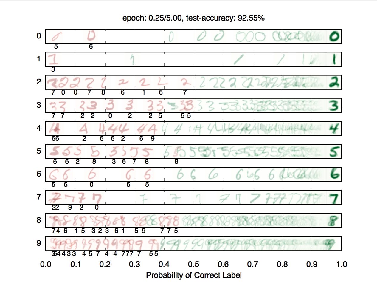
Question 3 (6 points): Digit Classification
For this question, you will train a network to classify handwritten digits from the MNIST dataset.
Each digit is of size \(28\times28\) pixels, the values of which are stored in a \(784\)-dimensional vector of floating point numbers. Each output we provide is a 10-dimensional vector which has zeros in all positions, except for a one in the position corresponding to the correct class of the digit.
Complete the implementation of the DigitClassificationModel class in models.py. The return value from DigitClassificationModel.run() should be a \(\text{batch_size} \times 10\) node containing scores, where higher scores indicate a higher probability of a digit belonging to a particular class (0-9). You should use nn.SoftmaxLoss as your loss. Do not put a ReLU activation after the last layer of the network.
For both this question and Q4, in addition to training data, there is also validation data and a test set. You can use dataset.get_validation_accuracy() to compute validation accuracy for your model, which can be useful when deciding whether to stop training. The test set will be used by the autograder.
To receive points for this question, your model should achieve an accuracy of at least 97% on the test set. For reference, our staff implementation consistently achieves an accuracy of 98% on the validation data after training for around 5 epochs. Note that the test grades you on test accuracy, while you only have access to validation accuracy - so if your validation accuracy meets the 97% threshold, you may still fail the test if your test accuracy does not meet the threshold. Therefore, it may help to set a slightly higher stopping threshold on validation accuracy, such as 97.5% or 98%.
To test your implementation, run the autograder:
python autograder.py -q q3
Question 4 (7 points): Deep Q-Learning
For the final project question of the semester, you will combine concepts from Q-learning and ML. In models.py, you will implement DeepQNetwork, which is a neural network that predicts the Q values for all possible actions given a state.
You will implement the following functions:
__init__(): Just like all other models, you will initialize all the parameters of your neural network here. You must also initialize the following variables:self.parameters: A list containing all your parameters in order of your forward pass.self.learning_rate: You will use this ingradient_update().self.numTrainingGames: The number of games that Pacman will play to collect transitions from and learn its Q values; note that this should be greater than 1000, since roughly the first 1000 games are used for exploration and are not used to update the Q network.self.batch_sizeThe number of transitions the model should use for each gradient update. The autograder will use this variable; you should not need to access this variable after setting it.get_loss(): Return the square loss between predicted Q values (outputted by your network), and the Q_targets (which you will treat as the ground truth).run(): Similar to the method of other models, you will return the result of a forward pass through your Q network. (The output should be a vector of size (batch_size, num_actions), since we want to return the Q value for all possible actions given a state.)gradient_update(): Iterate through yourself.parametersand update each of them according to the computed gradients. However, unlike all other models, you are not iterating over the entire dataset in this function, nor are you repeatedly updating the parameters until convergence. This function should only perform a single gradient update for each parameter. The autograder will repeatedly call this function to update your network.
Other than models.py, you will also need to implement the missing parts for the deep Q learning algorithm in compute_q_targets() for PacmanDeepQAgent in qLearningAgents.py.
Recall that the update rule for Q-Learning is \[Q(s,a) = Q(s,a) + \mathbf{\alpha}[r(s,a,s')+(1-done)\gamma\max_{a'}Q(s',a')-Q(s,a)] \]
So for the Q values to converge to optimal, it is necessary that:
\[[r+(1-done)\gamma \max_{a'}Q(s',a')]-Q(s,a)=0 \]In Deep Q Learning, we have 2 networks with the same architecture: a Q network \(Q(s,a)\) and a target network \(\hat{Q}(s,a)\). The task is to run regression to fit \(Q(s,a)\) to a target matrix which you compute in compute_q_targets().
The target matrix you return from this method should be of size (batch_size, num_actions), and should be first set equal to the Q network's prediction (please copy the values or strange things will happen).
Each row of the target matrix is a (1,num_actions) vector, and is the target computed from a transition \((s,a,r,s',done)\). We set its \(a\)-th entry \(target(s,a)=r+(1-done)\gamma \hat{Q}(s',\arg\max_{a'}Q(s',a'))+exploration\ bonus\), which basically means we still select the best action using Q network (\(a'=\arg\max_{a'}Q(s',a')\)), but we calculate the value using target network (\(\hat{Q}(s',a')\)).
The exploration bonus aims to encourage exploring more states and actions following this expression: \(exploration\ bonus=\frac1{2\sqrt{\frac{N(s)+1}{100}}}\) where \(N(s)\) is the number of times the agent visits that state. You can access this information in self.counts (a matrix that stores the counts in the corresponding x,y positions. \(N(s)+1=self.counts[x,y]\))
Sanity check: An example with batch_size=1, num_actions=2, legal_actions=[0,1,2,3]
Since batch_size=1, the input (the parameter) will only have one piece of transition \((s,a,r,s',done)\), and the output (target matrix) will be a 1 by 4 "matrix" (which is batch_size * num_actions*).
Suppose action \(a=2\), reward \(r=4\), \(done=False=0\), visit count \(N(s)=99\), discount factor \(\gamma=0.9\).
- First, we plug state \(s\) into the Q network and get \(Q(s,\cdot)=[10,20,30,40]\). (The dot means “for all 4 actions”)
- Then, we calculate the exploration bonus and get \(exploration_bonus=\frac1{2\sqrt{\frac{99+1}{100}}}=\frac12\).
- In order to get the next state's Q value, we plug next state \(s'\) into both the Q network and the target network and get \(Q(s',\cdot)=[5,6,7,8]\), \(\hat{Q}(s',\cdot)=[11,12,13,14]\). We pick the index with the maximum value for the Q network, which is index 3 having a max value of 8. In order words, \(\arg\max_{a'}Q(s',a')=3\). We then take the value in target network's output in that index, which is \(\hat{Q}(s',\arg\max_{a'}Q(s',a'))=\hat{Q}(s',3)=14\).
- We use the exploration bonus, the target network's output, and the reward to calculate the new Q value estimate \(target(s,a)=r+(1-done)\gamma\hat{Q}(s',\arg\max_{a'}Q(s',a'))+exploration\ bonus=4+(1-0)\times 0.9\times14+\frac12=17.1\).
- Finally, we set the values for the output target "matrix". All the values should first be copied from the Q network output, except for the action's entry being the new Q value estimate. So the matrix we return will be \(target=[10,20,17.1,40]\), the third entry (the action entry) is set to be 17.1.
- This target output is then sent to gradient_update() in the model to calculate mean square error with the Q network's output. So
loss=nn.SquareLoss([10,20,30,40], [10,20,17.1,40])\(=\frac14(0+0+(30-17.1)^2+0)\frac12=20.8\). (Don't worry about howSquareLossworks here.) And with this loss, we can perform back propagation to update our Q network.
When doing matrix operations, we should use numpy arrays instead of the Node class in this project. You can access the numpy matrix in the node by node.data. We've provided you all the variables in the mini batch: states, actions, rewards, next_states, and dones. Only states and next_states are "nodes" (in order to act as inputs for the neural networks), all other variables are numpy arrays. We've also provided a numpy version of states called states_np for your convenience when calculating the exploration bonus.
Some numpy functions you might need to look at include but not limited to: np.copy(), np.sqrt(), np.arange(), np.argmax(), and basic indexing in numpy matrix.
Try to use as many batched (vectorized) operations from numpy as possible instead of for loops over the samples to speed up learning.
Grading: You will get 3 points if you compute the targets correctly even if you don't have a good model. We will run your Deep Q learning Pacman agent for 10 games after your agent trains on self.numTrainingGames games. If your agent wins at least 6/10 of the games, then you will receive full credit. If your agent wins at least 8/10 of the games, then you will receive 1 extra credit. Please note that deep Q learning is not known for its stability, despite some of the tricks we have implemented in the backend training loop. The number of games your agent wins may vary for each run. To achieve the extra credit point, your implementation should consistently beat the 80% threshold.
python autograder.py -q q4
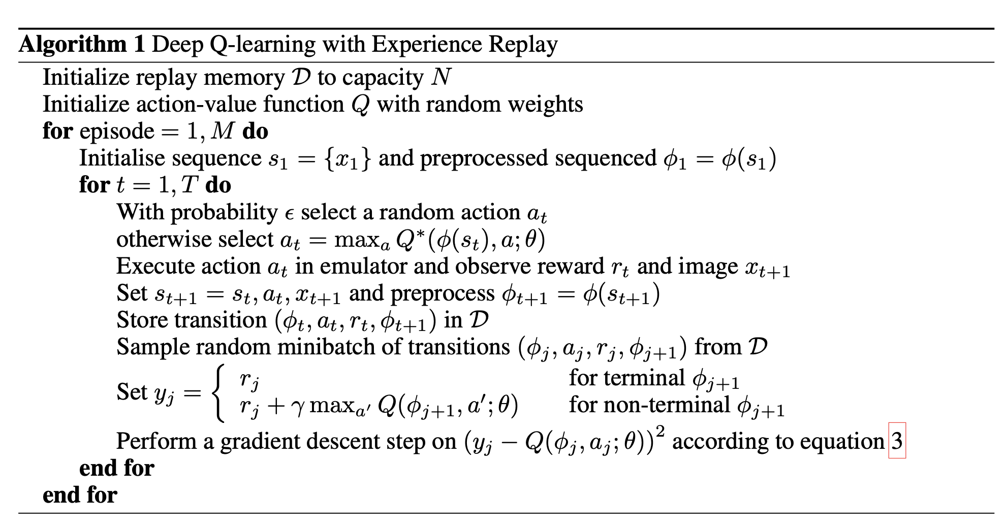
In case that you're interested in learning how Deep Q-learning works, here is some nice pseudocode from the famous DQN atari game paper on vanilla Deep Q-learning. Notice that we are NOT implementing this version of DQN in this project (in fact, many things are different) so don't use this paper as a reference. It's just here for you to see how deep Q-learning works besides the functions you implement. Here's another paper about Double Deep Q-learning (DDQN) which is more similar on what we're doing here (in terms of having two networks and etc.).
Congratulations! You have trained a deep RL Pacman and finished all the projects in 188! If you thought this was cool, try training your model on harder layouts:
python pacman.py -p PacmanDeepQAgent -x [numGames] -n [numGames + 10] -l testClassic
Submission
Submit machinelearning.token, generated by running submission_autograder.py, to Project 5 on Gradescope.
python submission_autograder.py
The full project autograder takes 2-12 minutes to run for the staff reference solutions to the project. If your code takes significantly longer, consider checking your implementations for efficiency.
Note: You only need to submit machinelearning.token, generated by running submission_autograder.py. It contains the evaluation results from your local autograder, and a copy of all your code. You do not need to submit any other files.
Please specify any partner you may have worked with and verify that both you and your partner are associated with the submission after submitting.
Congratulations! This was the last project for CS 188!