 Original
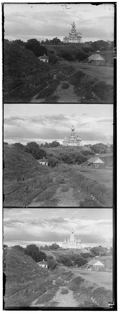
The objective of the project was to create a colorized image from three separate images, each taken with a red, green, or blue filter. Glass plate negatives of these images, taken by Sergei Mikhailovich Prokudin-Gorskii (1863-1944), were preserved by the Library of Congress and were recently made available online. For this project, our task was to, for each image, efficiently extract its three separate color channel images and align them on top of each other so that the resulting photo depicts the original photograph with a minimal amount of visual artifacts.
Original
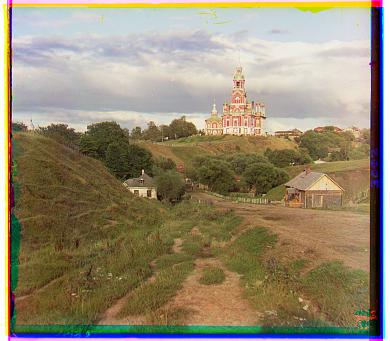 Colorized
I divided the colorizing process itself into 3 separate tasks: separating the different color channel images, aligning the images, and then
stacking the images together. Separating the color channels simply involved dividing the original file's height by 3, and then
assigning each BGR plate to the top, middle, or bottom third of the file (respectively). This created the three separate images
needed to colorize the photograph. Additionally, stacking the images together at the end was just as simple, using the
dstack numpy method. Aligning the images was a much trickier process.
NCC Approach: To align the JPEG images, I calculated the NCC (normalized cross-correlation)
values between the shifted blue and red plates and the green plate (our reference plate). I calculated the NCC across a displacement
range of [-15,15] for both horizontal and vertical shifts, and chose the displacement with the highest NCC in respect to the green plate. The resulting shifted plates
would be used to create the final aligned image. When initially running this algorithm, I noticed that the borders of each
plate could possibly interfere with the NCC values, as many of the photographs have a black or white border that is not
part of the actual picture itself. To account for this, I only calculated the NCC on the inner 2/3 of each image,
meaning 1/6 of the photo is cropped from each edge. However, the final image is made using the uncropped version of each photo.
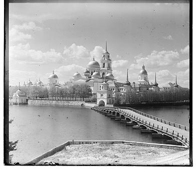 Original
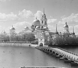 Cropped for NCC
Image Pyramid: For the TIFF images, the range of possible displacements is much larger, as the files
themselves are at least 10 times larger than the JPEG images. Instead of running the same algorithm as above with a much
larger displacement range, a more efficient way to find these displacement values was to use an image pyramid. For each
TIFF file, I resized each color channel image by 0.5 until it was less than 500 pixels high (about the size of a JPG file). I then aligned
this image using the NCC approach described above, using the [-15,15] displacement range. Then, using the resulting displacement (x,y) for the
smallest image, I recursively ran the alignment algorithm on the second smallest image, with a displacement range of
[x*2-2, x*2+2] for horizontal shifts and [y*2-2,y*2+2] for vertical shifts. I repeated this again and again using recursive calls until
the displacement for the original image is found. This strategy allows for a smaller, more accurate range of possible displacements,
and creates a much more efficient runtime.
Blue displacement: (-5, -2), Red displacement: (7, 1)
 Blue displacement: (3, -2), Red displacement: (6, 1)
 Blue displacement: (-3, -1), Red displacement: (4, -1)
 Blue displacement: (-7, 0), Red displacement: (8, -1)
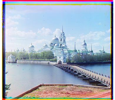
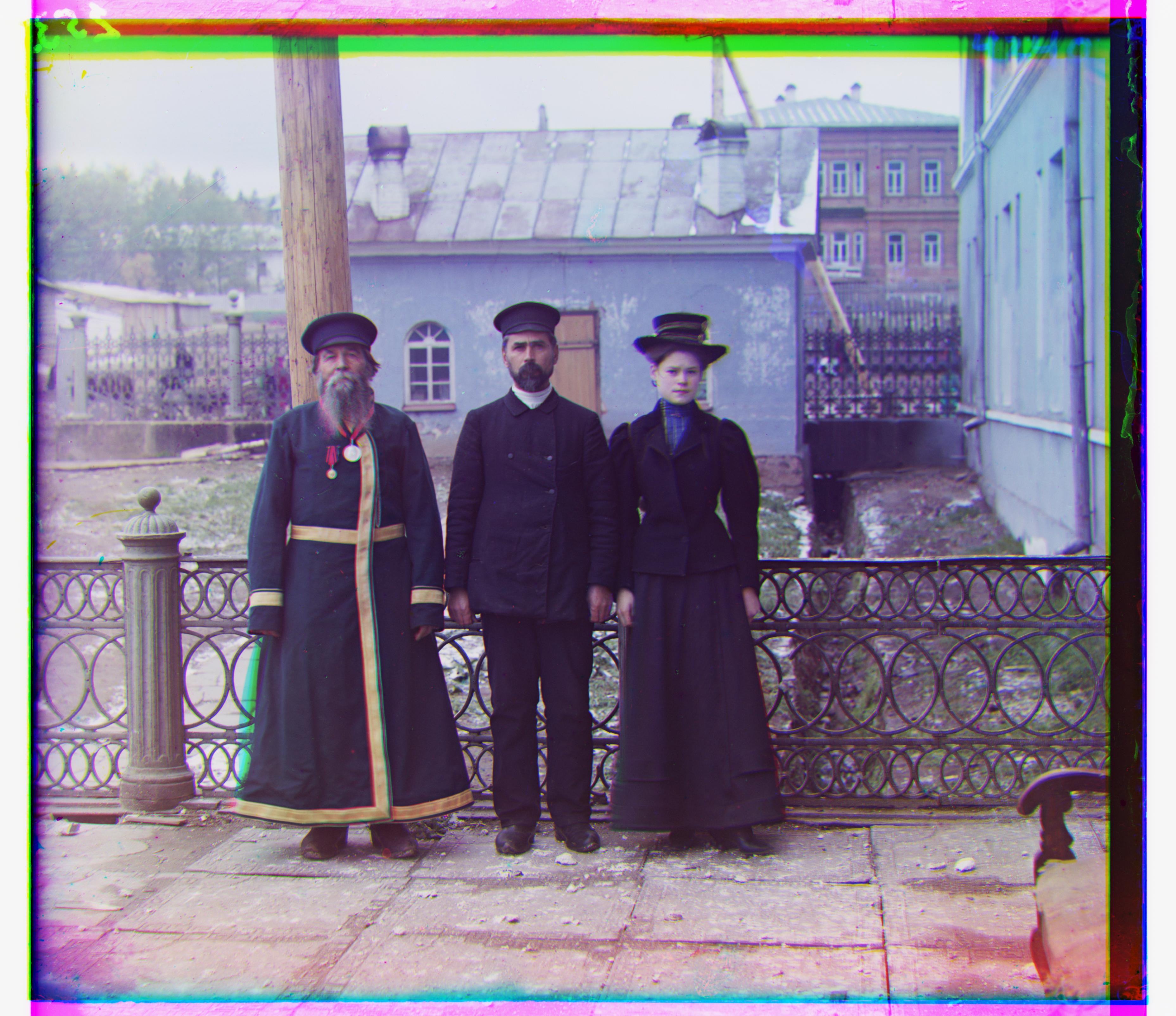
 Blue displacement: (-26, -46), Red displacement: (14, 54)
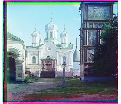
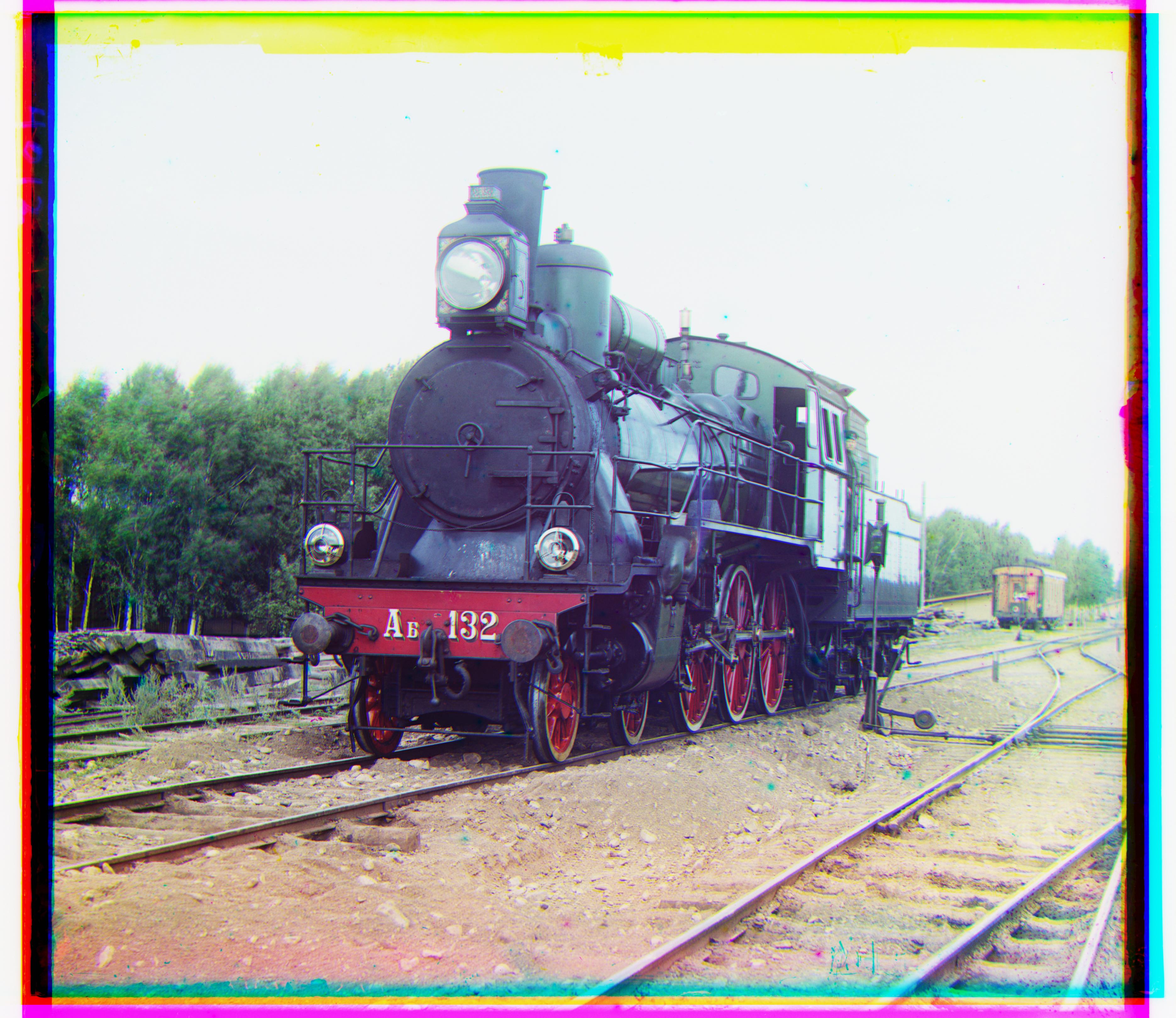
 Blue displacement: (-18, -58), Red displacement: (-2, 62)
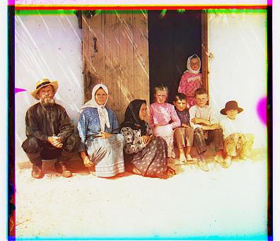
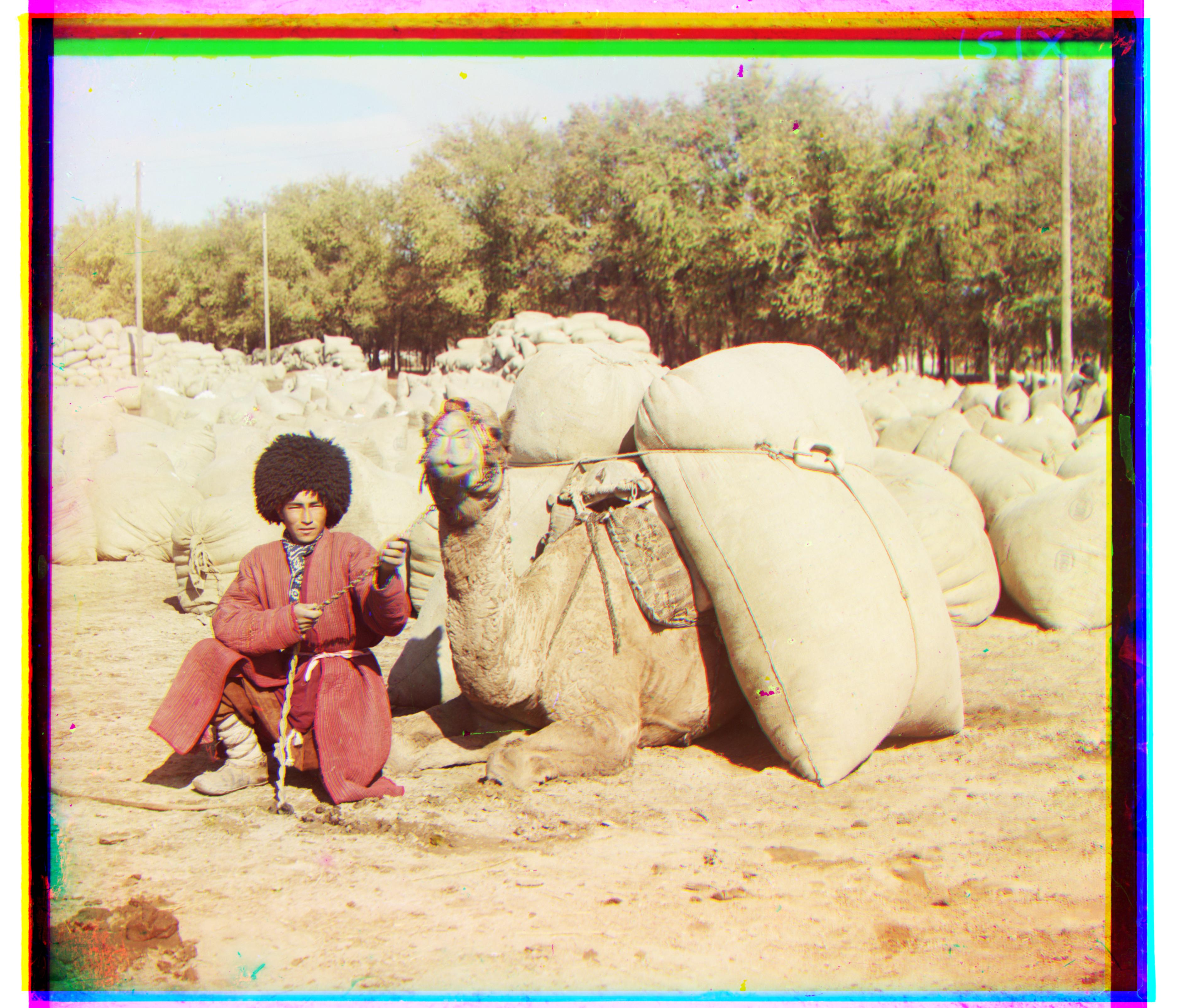
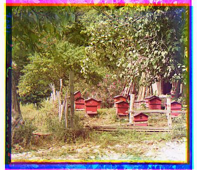
![]() Blue displacement: (-18, -38), Red displacement: (6, 46)
Blue displacement: (-18, -38), Red displacement: (6, 46)
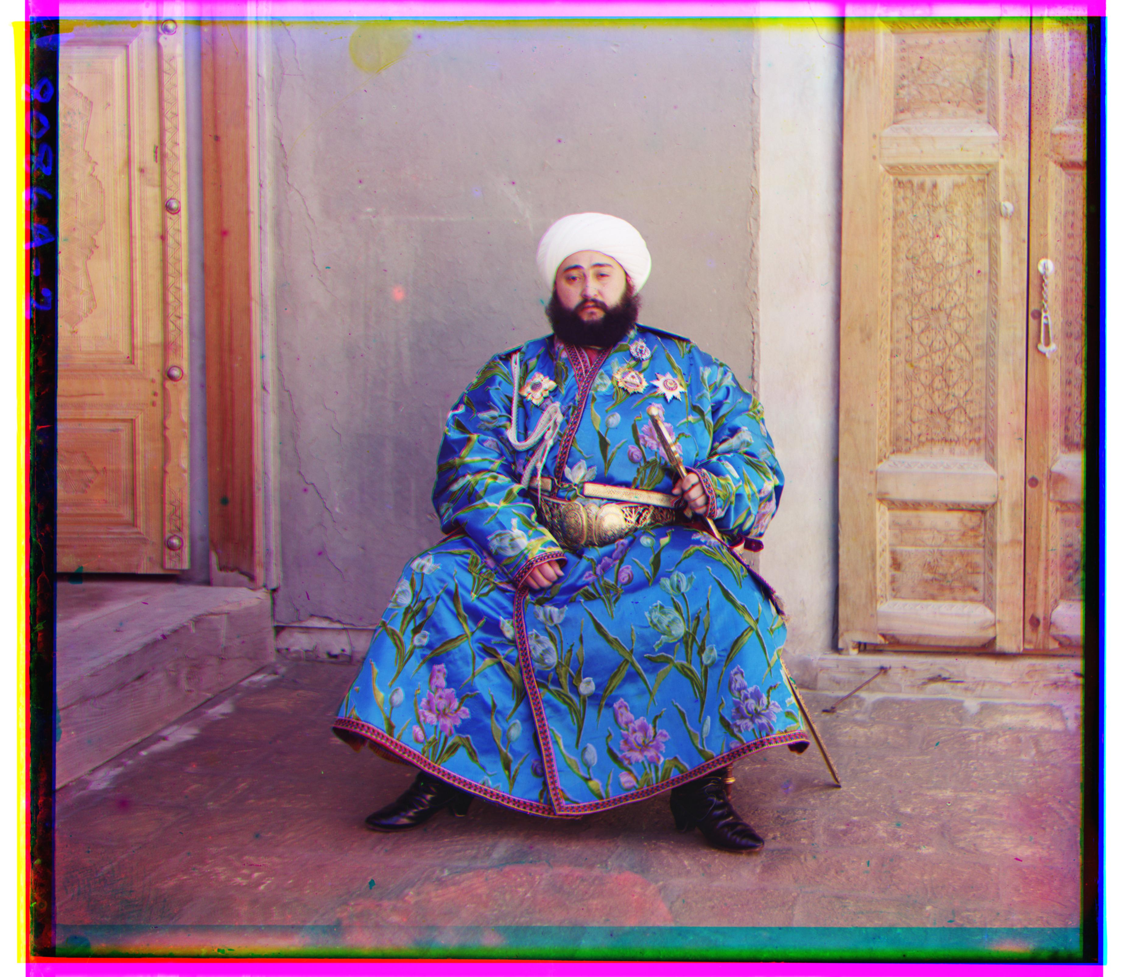
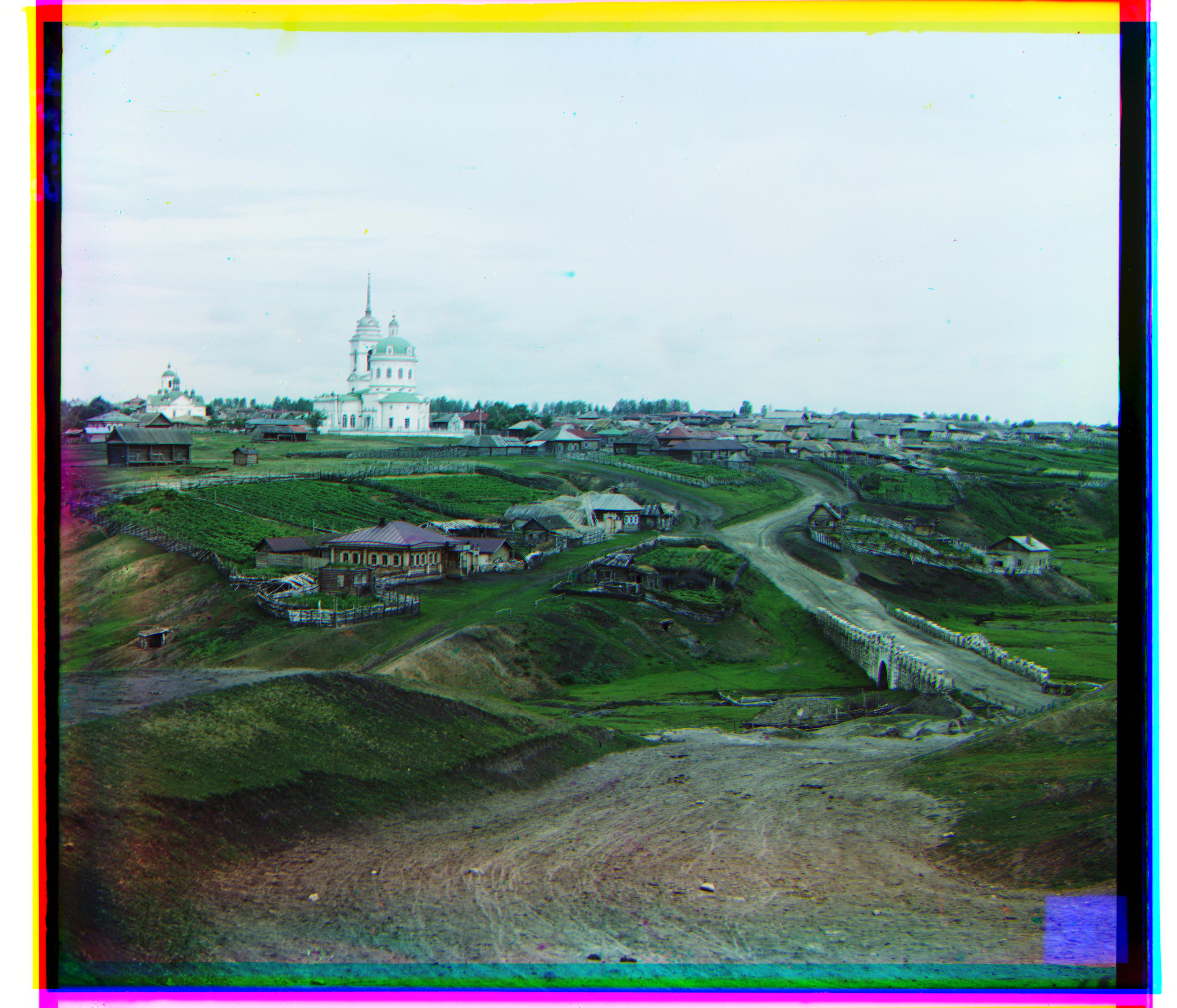
 Blue displacement: (-10, -50), Red displacement: (6, 58)
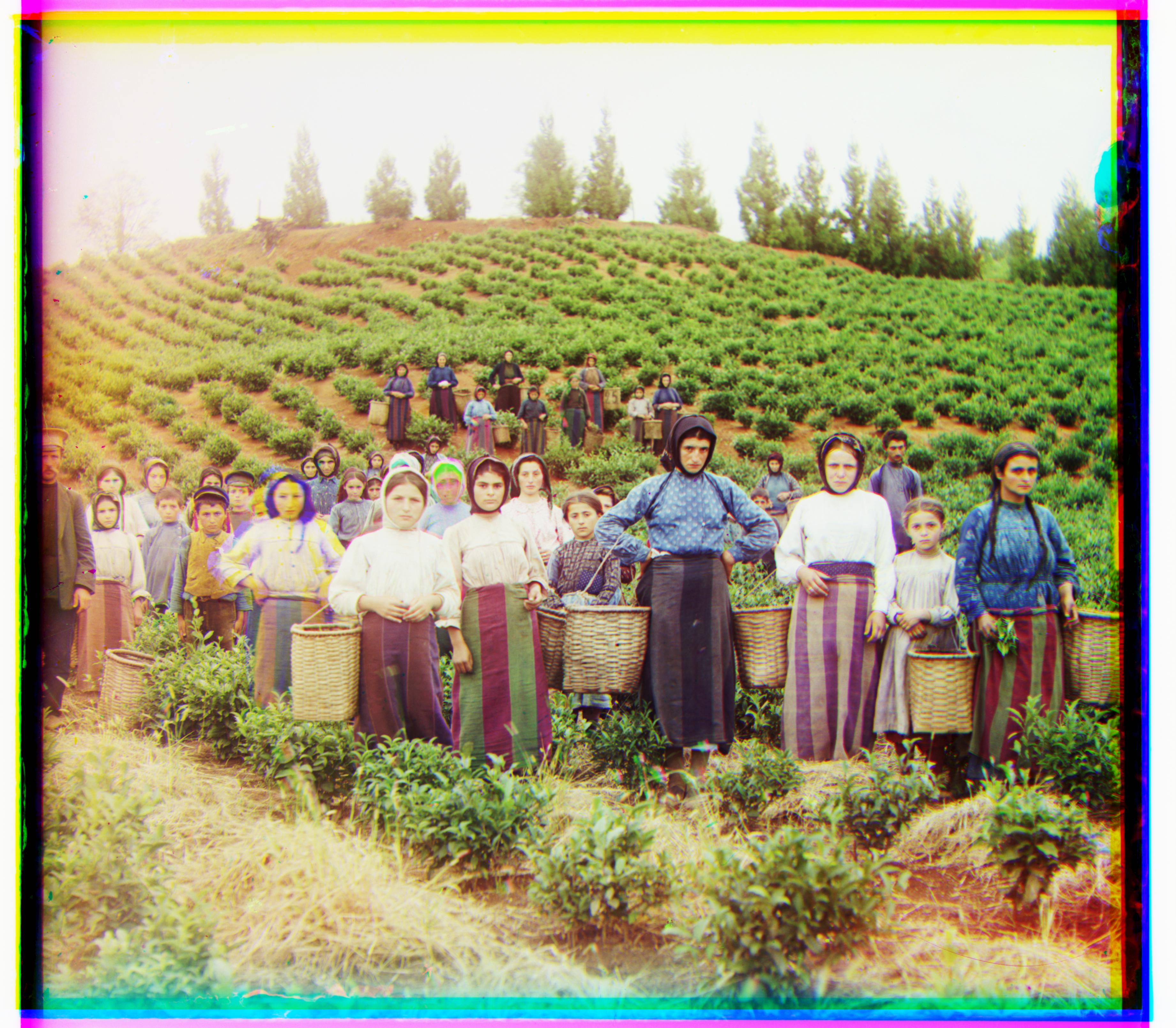
 Blue displacement: (-22, -58), Red displacement: (6, 70)
 Blue displacement: (-30, -78), Red displacement: (10, 94)
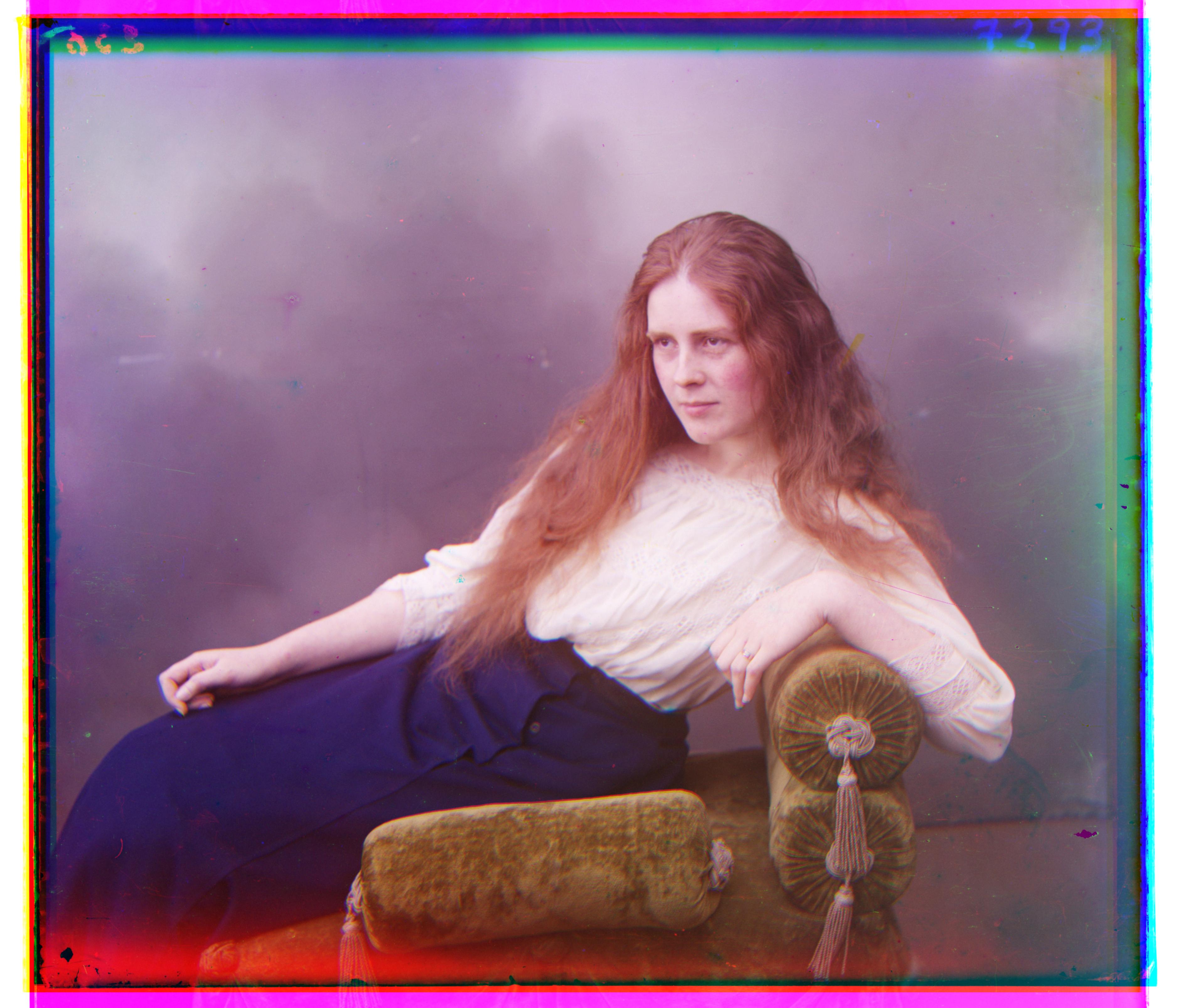
 Blue displacement: (-14, -50), Red displacement: (-2, 58)
 Blue displacement: (-6, -42), Red displacement: (30, 42)
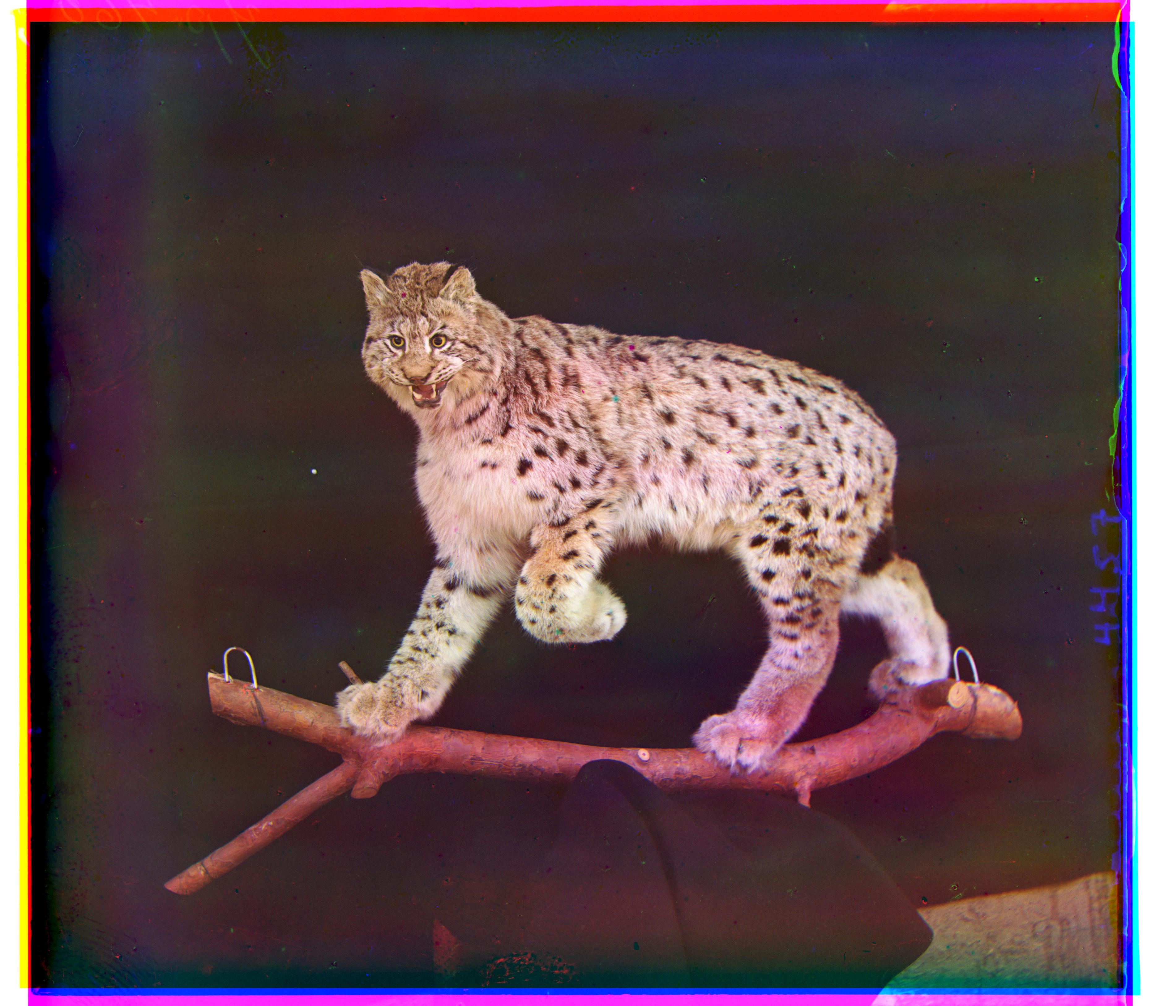
 Blue displacement: (-22, -54), Red displacement: (10, 58)
 Blue displacement: (-10, -62), Red displacement: (14, 70)
 Blue displacement: (-11, -4) Red displacement: (12, 2)
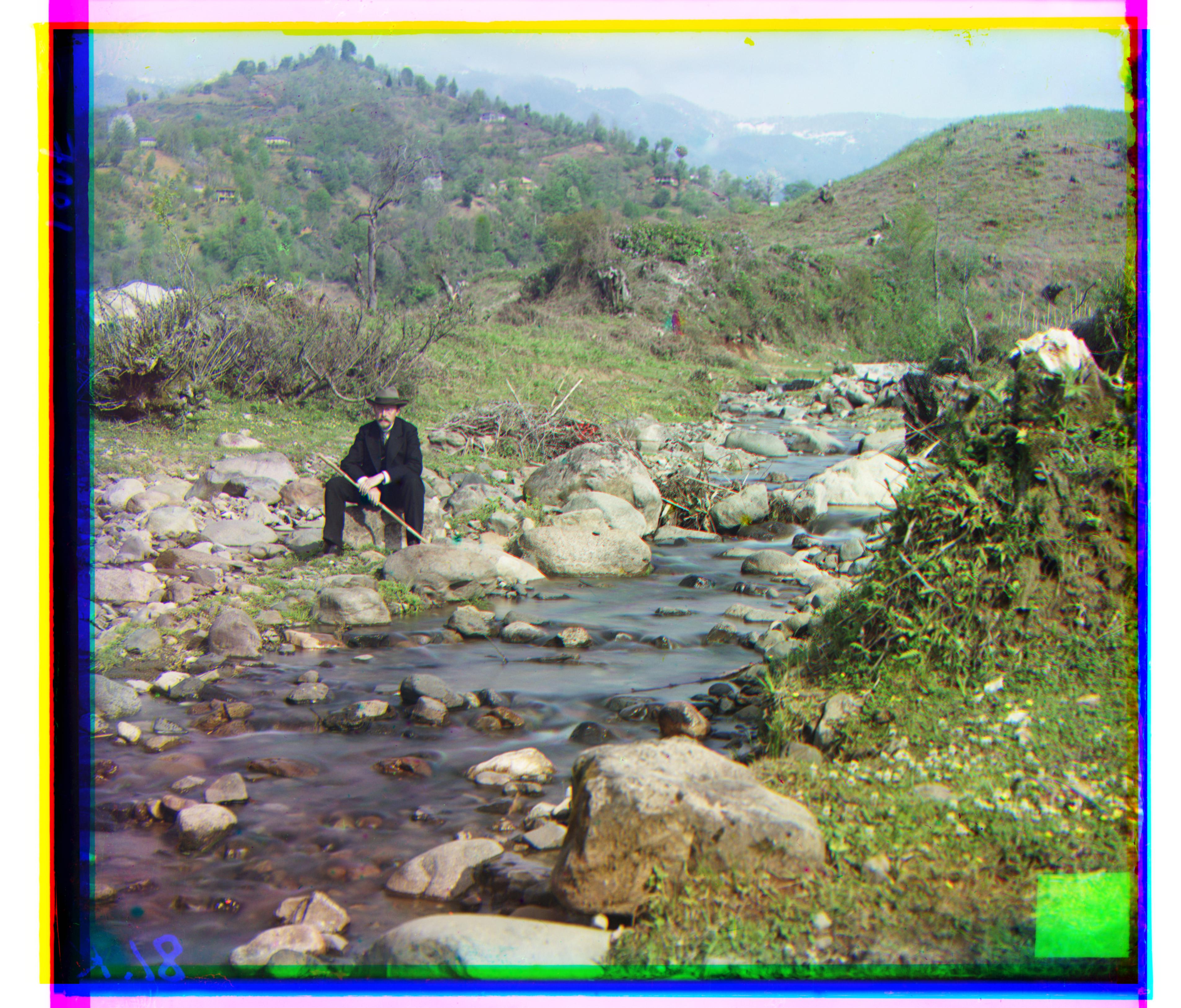
 Blue displacement: (-10, -18), Red displacement: (10, 66)
 Blue displacement: (10, -42), Red displacement: (-10, 90)
Both the simple NCC approach and the image pyramid seemed to work extremely well. Surprisingly, I was able to make
the window of displacement for the image pyramid extremely small, with a range of only 5 pixels for both horizontal and
vertical shifts. This means that rescaling the image and running NCC on the JPG-size image is fairly accurate to
begin with.