
Baseline - Brute force alignment
I built a baseline alignment method to use for comparison against other methods. The baseline checked a neighborhood of possible different color channel alignments. I translated the image in a range of [-20, 20] for both the x and y coordinates, aligning the green and blue channels with the red channel. I measured alignment by using two different metrics - Normalized Cross Correlation and the L2 Norm (also known as Sum of Squared Differences (SSD). At first, I calculated these metrics across the entire image. After a few failed alignments, I realized that the borders of the image occasionally seemed to hurt the quality of the metric - thus I decided to use a window of the image that kept the center 2/3 and ignored the borders. This alignment method provides a great baseline. It works very quickly on the smaller images, each of which are approximately 400x300 pixels.Experimental Details
I analyzed two different translation techniques and two different alignment metric for this portion of the project. For translation, I tried using the np.roll function as well as np.pad and observed the resulting images.Focuse on center of images
Originally, I did not crop the image while calculating any of the metrics. This lead to unfortunate effects where the edges of hte image, which sometimes contained extra noise, writing, and inconsistent weathering, would lead to faulty alignments. To fix this issue, I only used the center 2/3 of the image, as displayed below.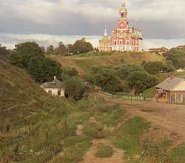


Translation
The np.roll function takes in a matrix and the vector of translation and then shifts the matrix according to the vector. Any elements of the matrix that are pushed out of the orignal matrix frame by the translation vector are placed immediately on the other side of the matrix. This is the method that was originally suggested, however I wondered if it would be better to pad with zeros instead of rolling the vectors off of the edges. That's why I implemented the np.pad based translation. The motivation here is that np.pad would fill in the missing gaps not with the rolled over elements, but rather zero padding. I believed that this would help with the alignment metric alignment procedure because it wouldn't add extra information on the sides of the image that could potentially negatively impact the quality of the metric. However, on testing I found that this did not actually effect the metric, especially after I added the metric image cropping mentioned above.Metrics
As mentioned above, I employed two metrics for this first baseline : Sum of squared differences and Normalized Cross Correlation.Sum of Squared Differences
The sum of squared differences is the simplest metric of the two and measures the raw difference between pixels in an image. The formation is as so, given two vectorized representation of channels, $c_1$ and $c_2$, the sum of squared differences is simply $$ \text{SSD}(c_1, c_2) = \sum_{i} (c_1[i] - c_2[i])^2$$ which is the same as the L2 Norm. To find an optimal alignment, our objective is to minimize the SSD between two target channels. An SSD of 0 means that the pixel intensities are identical.Normalized Cross Correlation
The normalized cross correlation metric (NCC) uses a different metric that instead uses properties of inner products to measure similarity. NCC is defined below $$\text{NCC}(c_1, c_2) = \left(\frac{c_1}{ \|c_1\|}\right )^T \cdot \frac{c_2}{ \|c_2\|}$$ The basic idea is that two vectors that are identical will have an NCC of 1, while two completely dissimilar images (aka orthogonal) will have an NCC of 0. The objective thus becomes to maximize the NCC. I took the original NCC formulation above and tweaked it slightly to reuse the minimization componnents that I built for SSD. I simply took the inverse of NCC, yielding an objective that should be minimized rather than maximized. $$ \text{NCC}_{tweak}(c_1, c_2) = \frac 1{\text{NCC}(c_1, c_2)}$$Comparison

Results
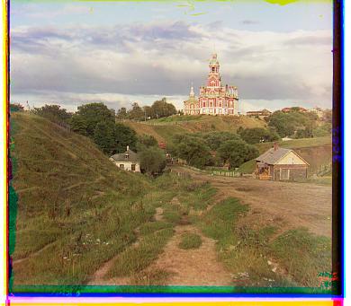
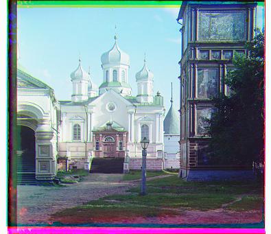
Now we showcase the results across for the remaining small images. We compare the image aligned with SSD on the left with NCC on the right.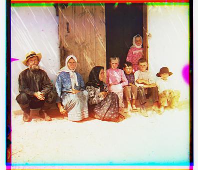


Pyramid Alignment
Brute force alignment works very well for all of the images small images above, however for higher quality images that are 3700x3000 px, this method falls apart. We'd have to search over a set of translations far larger than [-20, 20], and the 10x larger image will increase the amount of time necessary to calculate the metric as well.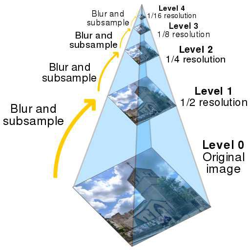
#/media/File:Image_pyramid.svg)
Therefore, I took a different approach by utilizing what is known as an Image Pyramid. An image pyramid is a technique commonly used for many different image processing purposes. In my implementation, I began running brute force alignment at a very coarse scale (or in otherwords, when the image is resized to be rather small). This gave me a rough estimate of where the translation should be. Then, I'd take a more fine scale image, rescale the translation found at the previous scale, then use this rescaled translation as the starting point for another brute force alignment. I repeated this process, doubling the scale until I reached the original image and run a final brute force alignment.
Cost function Evaluation
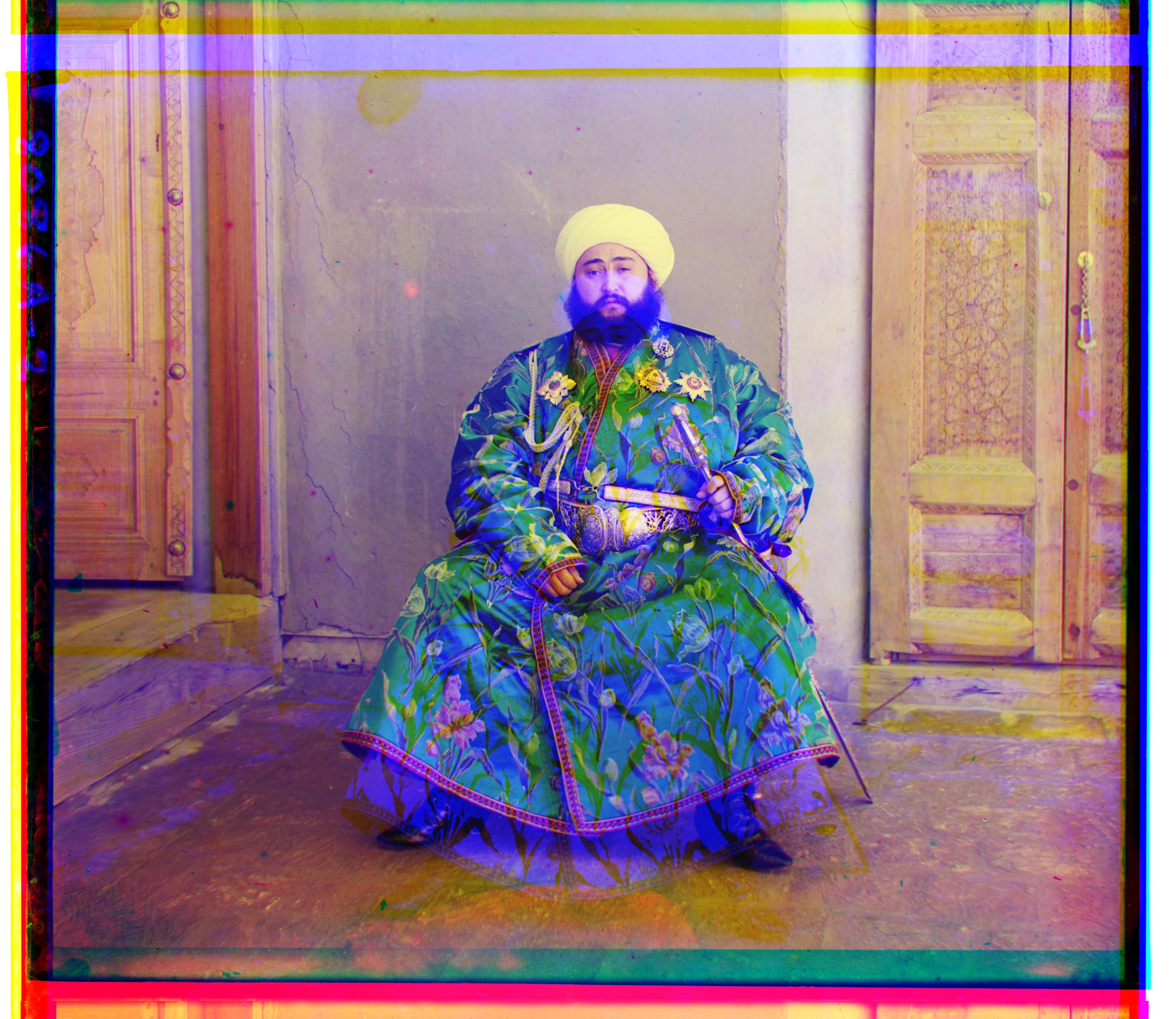
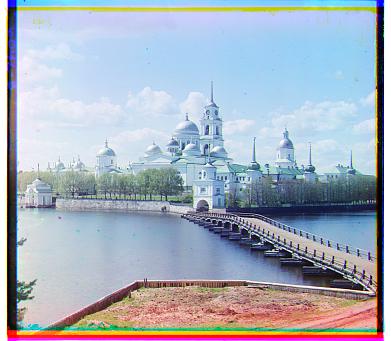
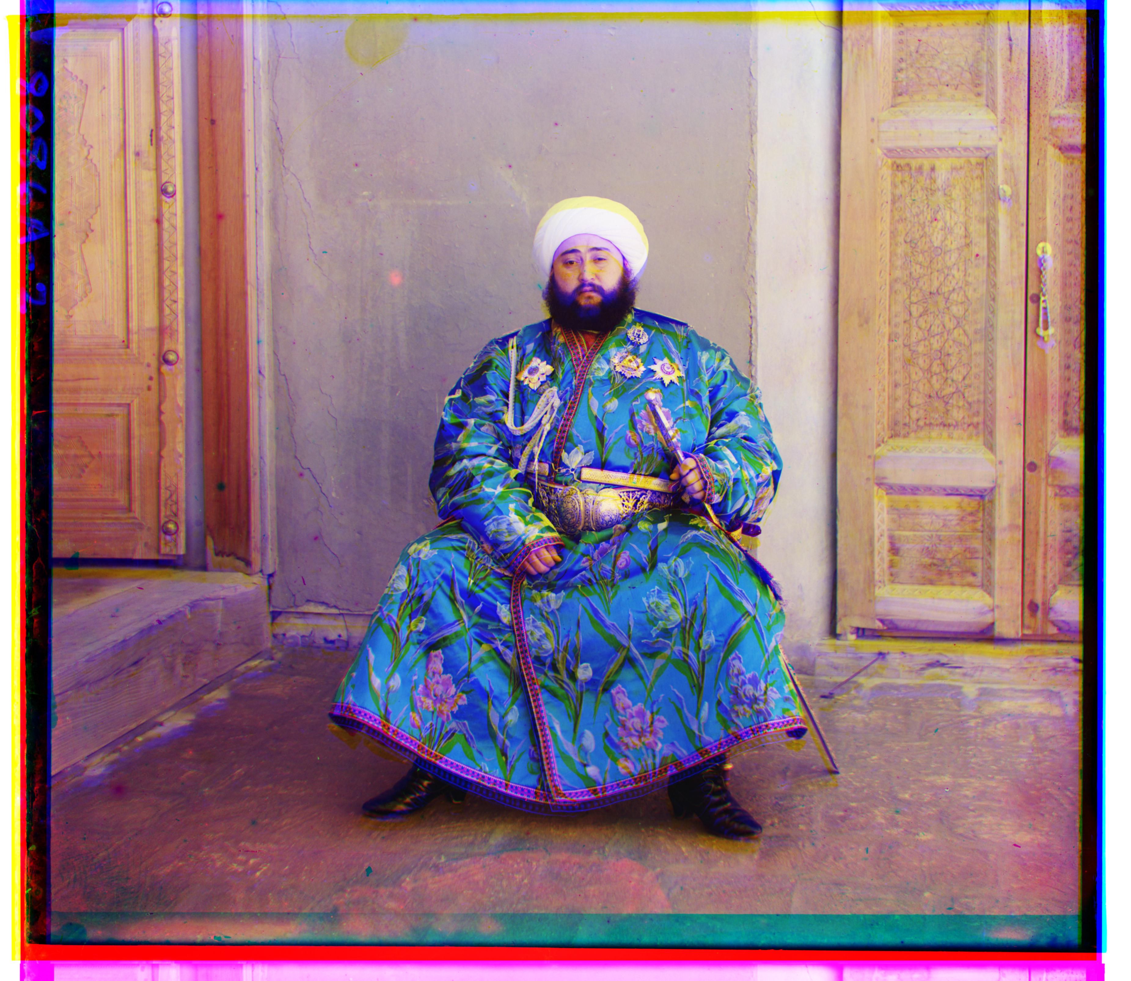
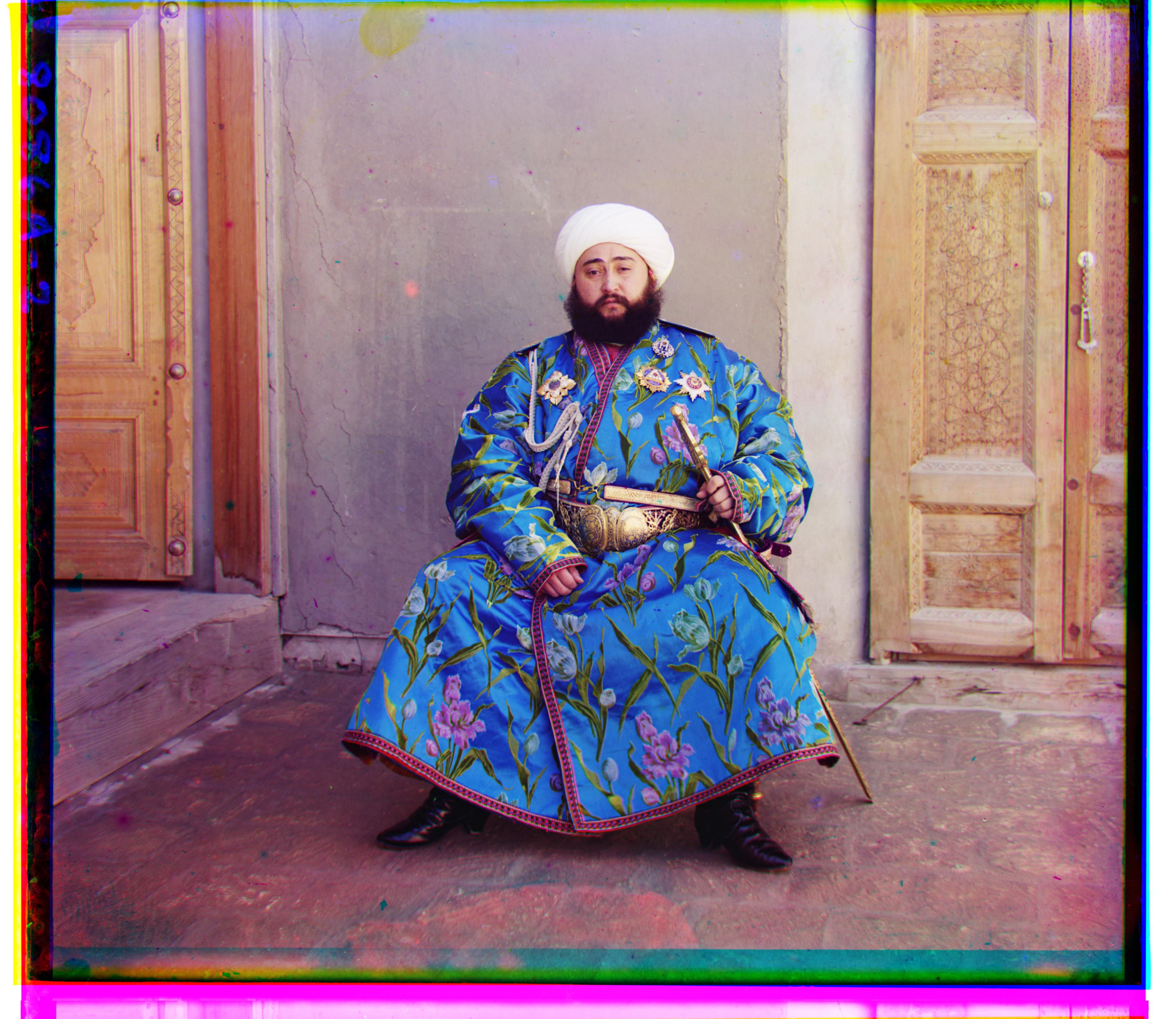
I ran both the NCC and SSD cost functions for pyramid alignment, and both appeared to perform very well. In Piazza, there were many mentions that the alignment algorithm had issues with the Emir photograph, displayed below. However, on my runs, there appear to be no differences in the images, and there are barely any differences in channel shifts -- if there is any at all.


Results
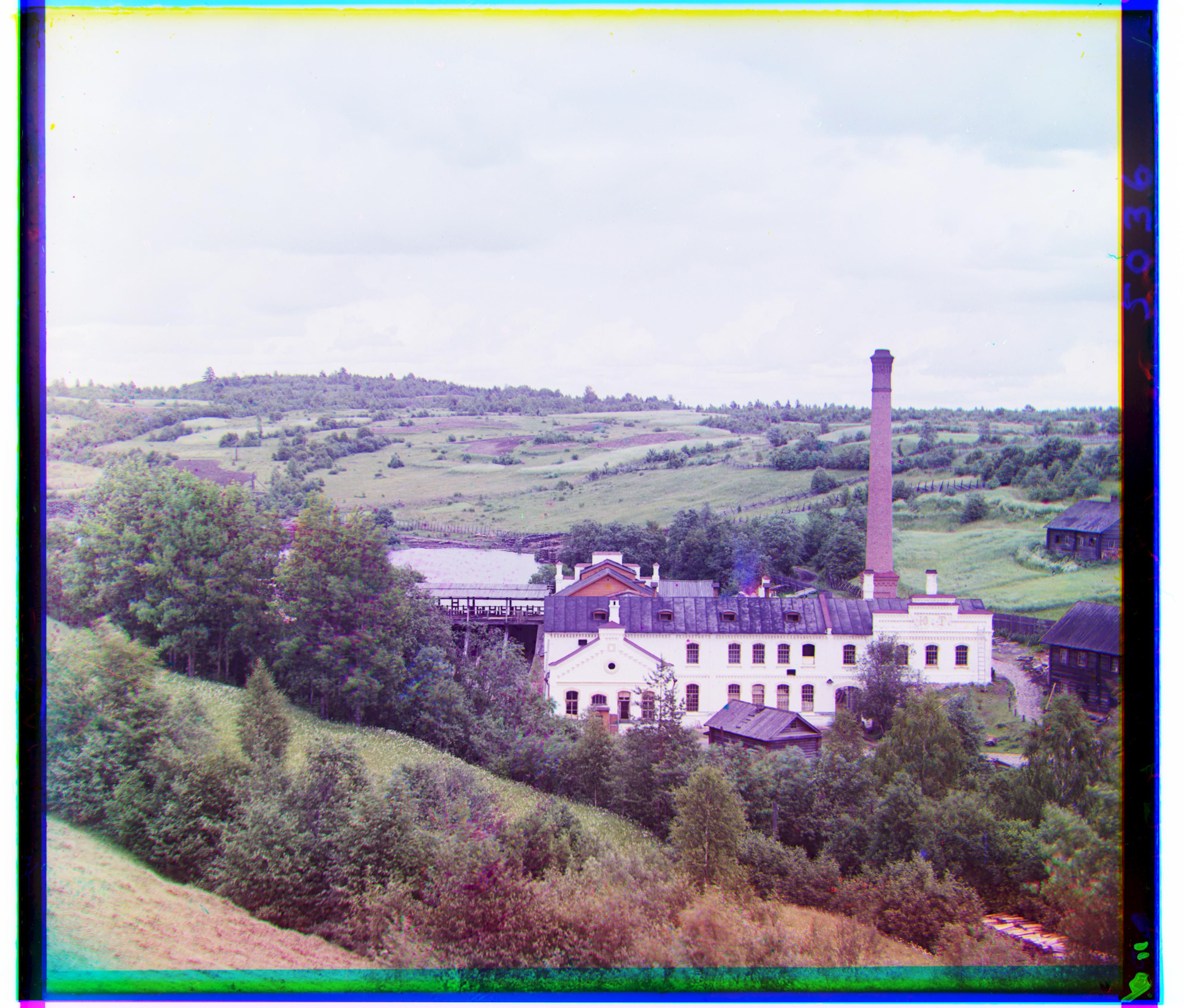
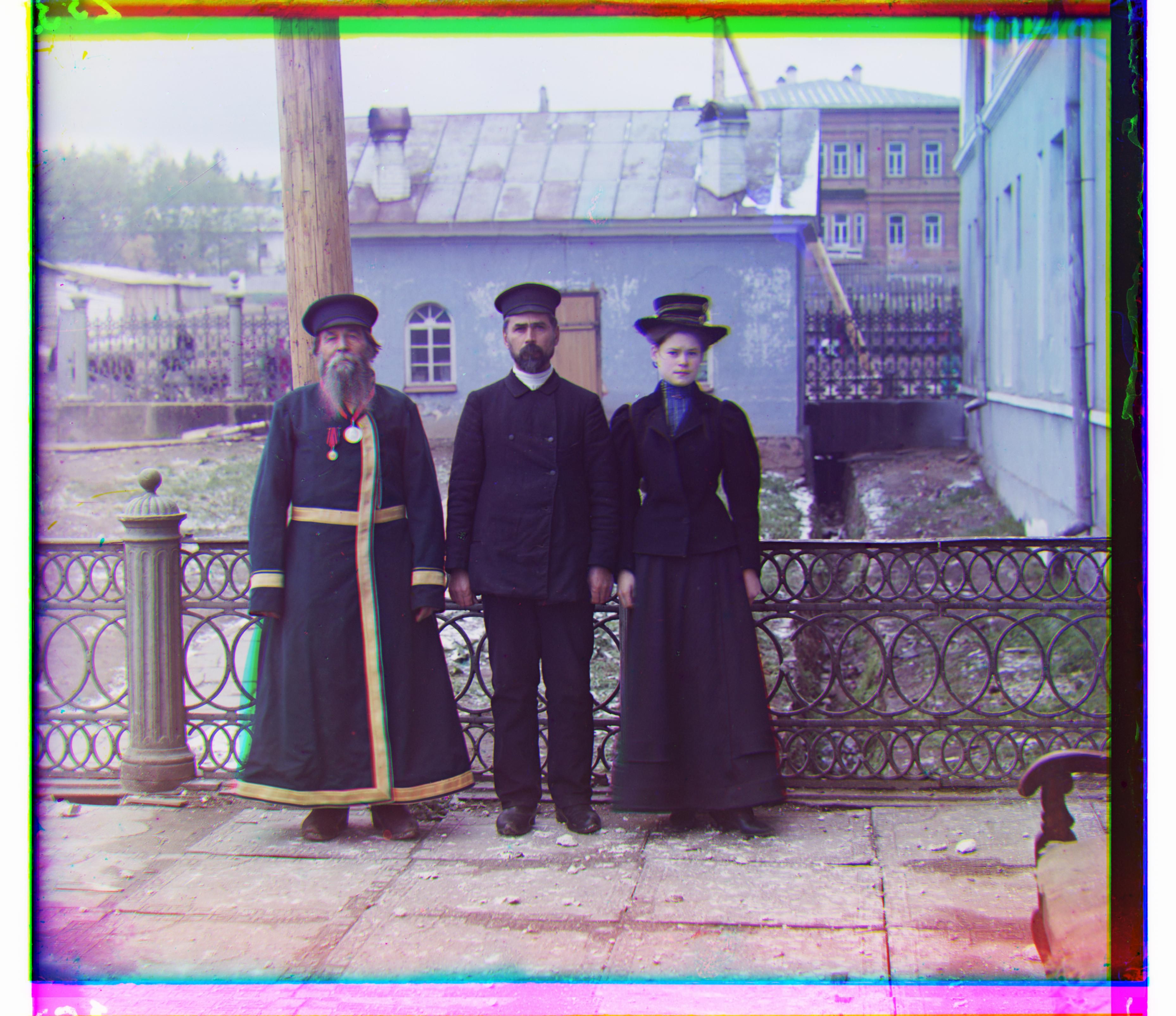
Here we output the aligned images using NCC as the cost function and an Image Pyramid for alignment.

Bells and Whistles
Edge Detection
For my bells and whistles, I focused on edge detection for alignment. As a baseline, I used a sobel filter which was suggested on piazza and was rather easy to implement. For the fun of it and buying into the hype, I also wanted to use a completely different edge detector - the first layer of a convolutional neural network.Sobel Filter
Sobel edge detector simply convolves two different $3\times 3$ filters on an image, which are reproduced belowSobel Results

Learned filter
As a challenge for myself, I wanted to see if I could ride the deep learning hype train into my cs194 homework. Convolutional neural networks are the powerhorse of the deep learning revolution. A convolutional neural network is composed of a series of convolutional layers - a set of convolutional kernels that are adjusted during the training of the network. These weights are adjusted so as to maximize an objective, say classifying a wide range of possible images, as is the case of the ILSVRC competition. If you're interested in learning more about CNNs, I recommend checking out the Stanford course on Deep Learning and enroll in the Deep Learning Decal next semester! On analysis of the filter responses of the first layer, the first layer ends up learning filters that are basically specialized edge detectors. That is why I thought a neural network might be an interesting tool to use to extract edges - I figured the filters used by the network will likely be much more encompassing than a simple Sobel filter. For this filter, I used the first layer of a VGG net trained on ImageNet. This model was trained by the developers of the Keras Deep Learning Library and available as a part of the api. I noted that filters normally traversed all the way through the channels of a colored image. To resolve this issue, I grabbed the slice of the filter corresponding to the specific channel that I wished to align. There are a total of 64 filters for this first convolutional layer. I ended up timing runtime, and was not satisfied with the roughly 16 second runtime for convolving. I decided to skip optimization past the scipy.convolve algorithm (mainly because I was running out of time for submission), and instead take a subset of the filters for aligning the images.Results