For smaller images, a naïve algorithm could be done to analyze the best color combination. For this algorithm, the blue channel was not displaced to any extent. Specifically, the green-filtered and red-filtered images were aligned to the blue-filtered images. Both the green and red-filtered images were displaced up to 15 pixels in the negative and positive x and y direction. But how do we determine which displacement will produce the best color combination? Simply put, the Sum of Squared Differences (SSD) is utilized.
For each displacement, the Sum of Squared Differences (SSD) between the displaced images (red, green) and our base image (blue) was calculated. The amount of displacement that produced the smallest SSD was calculated. Then, the shifted red and green-filtered images were aligned with the original, blue-filtered image. The result is the colored image.
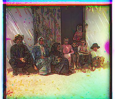
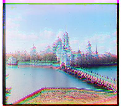
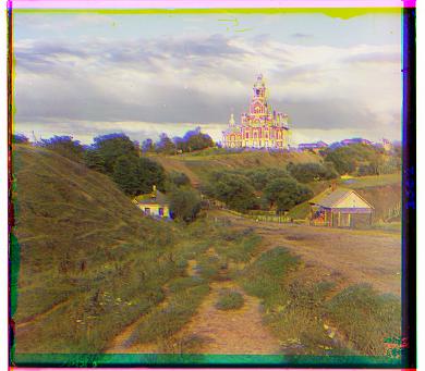
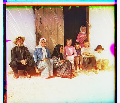
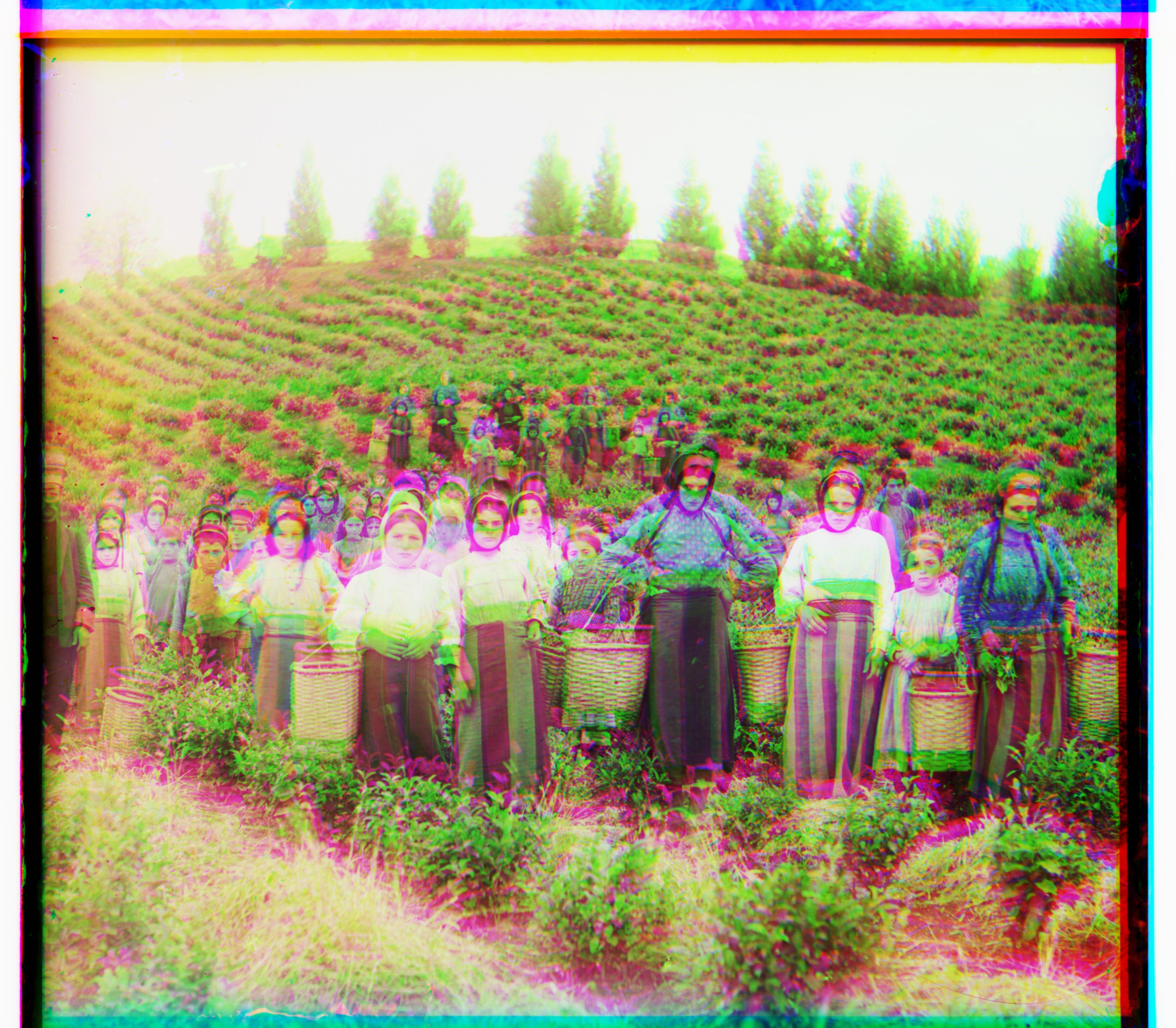
Here are the images!
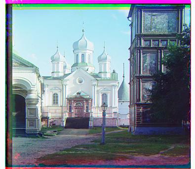
Images are here
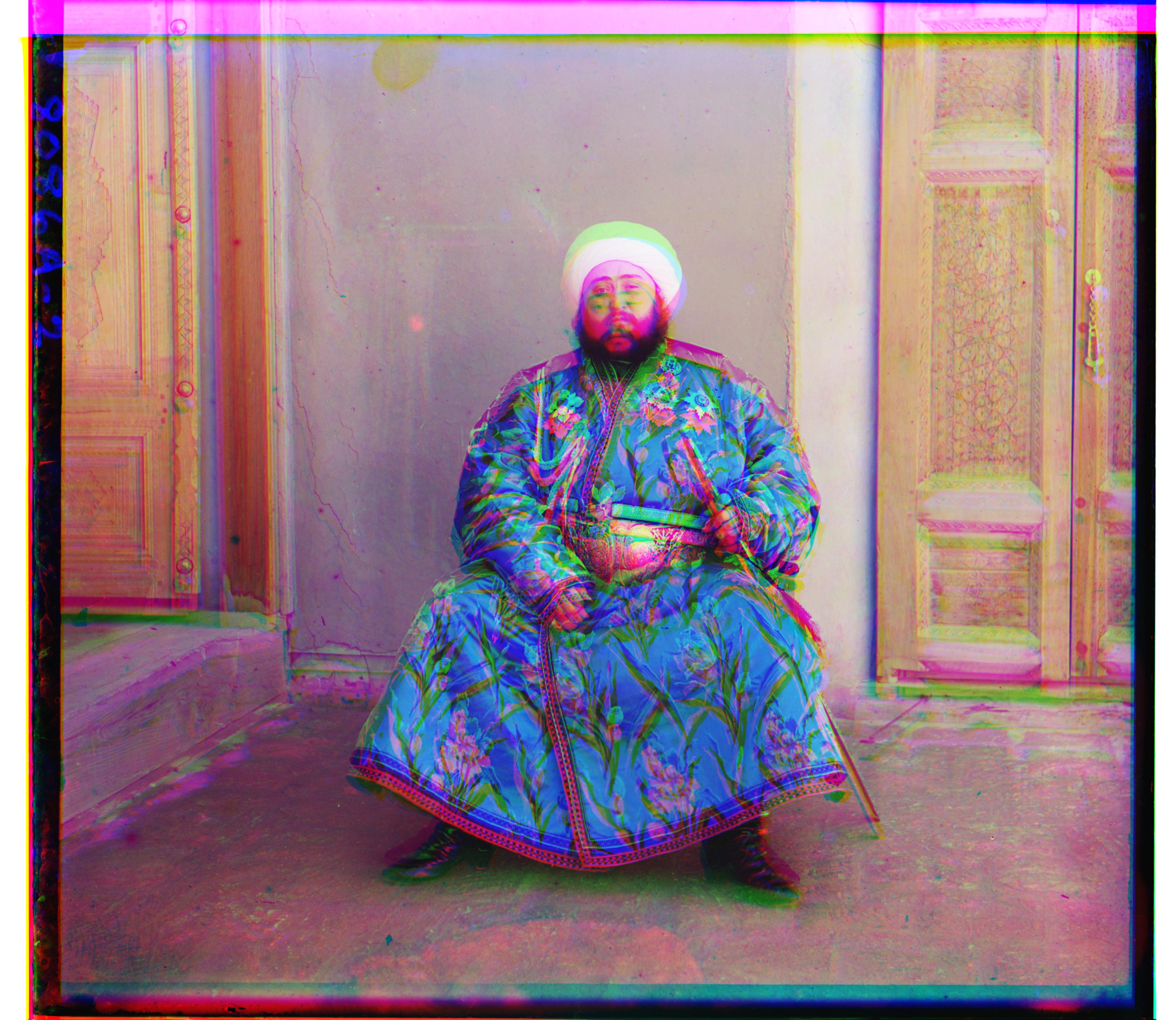
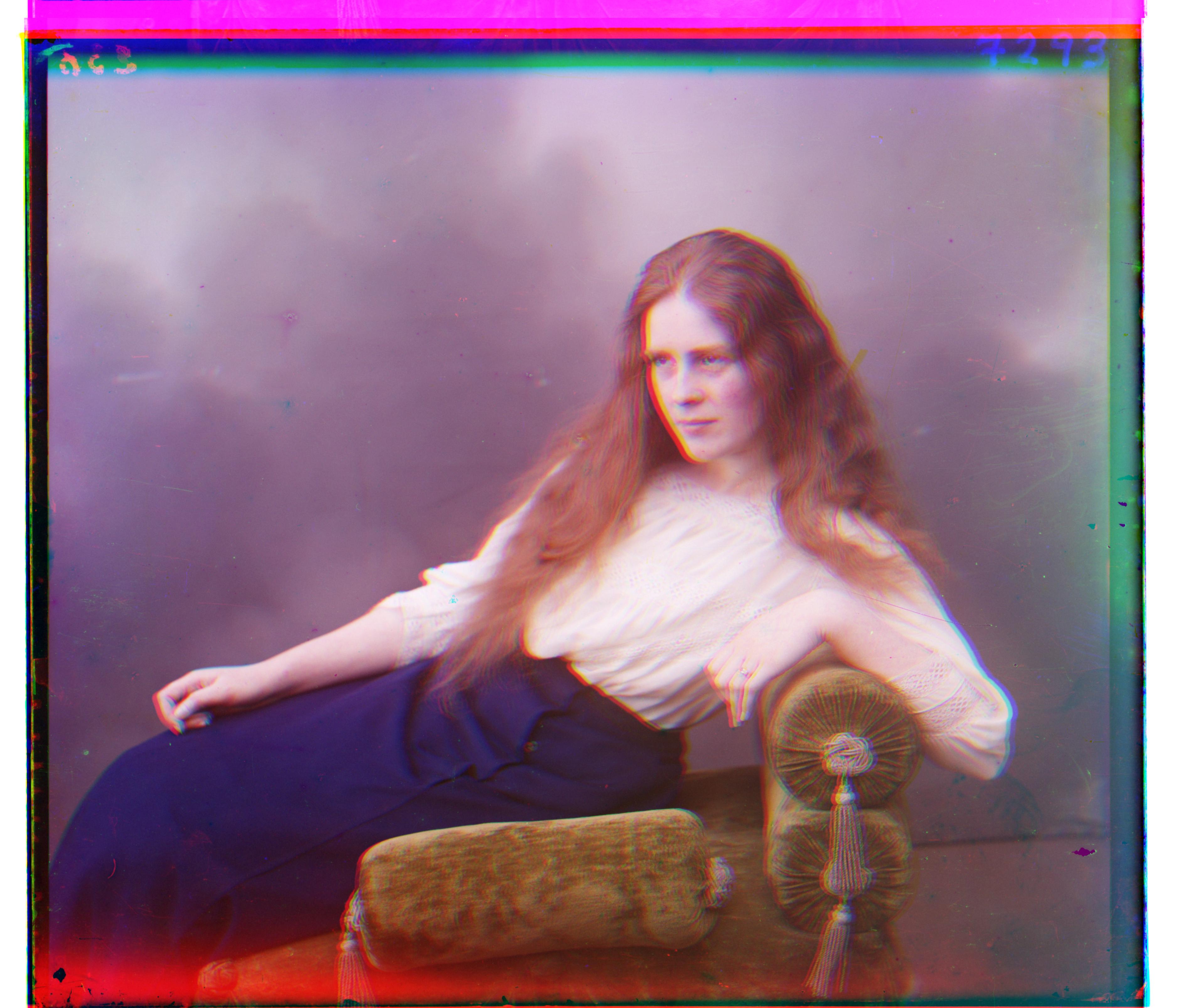
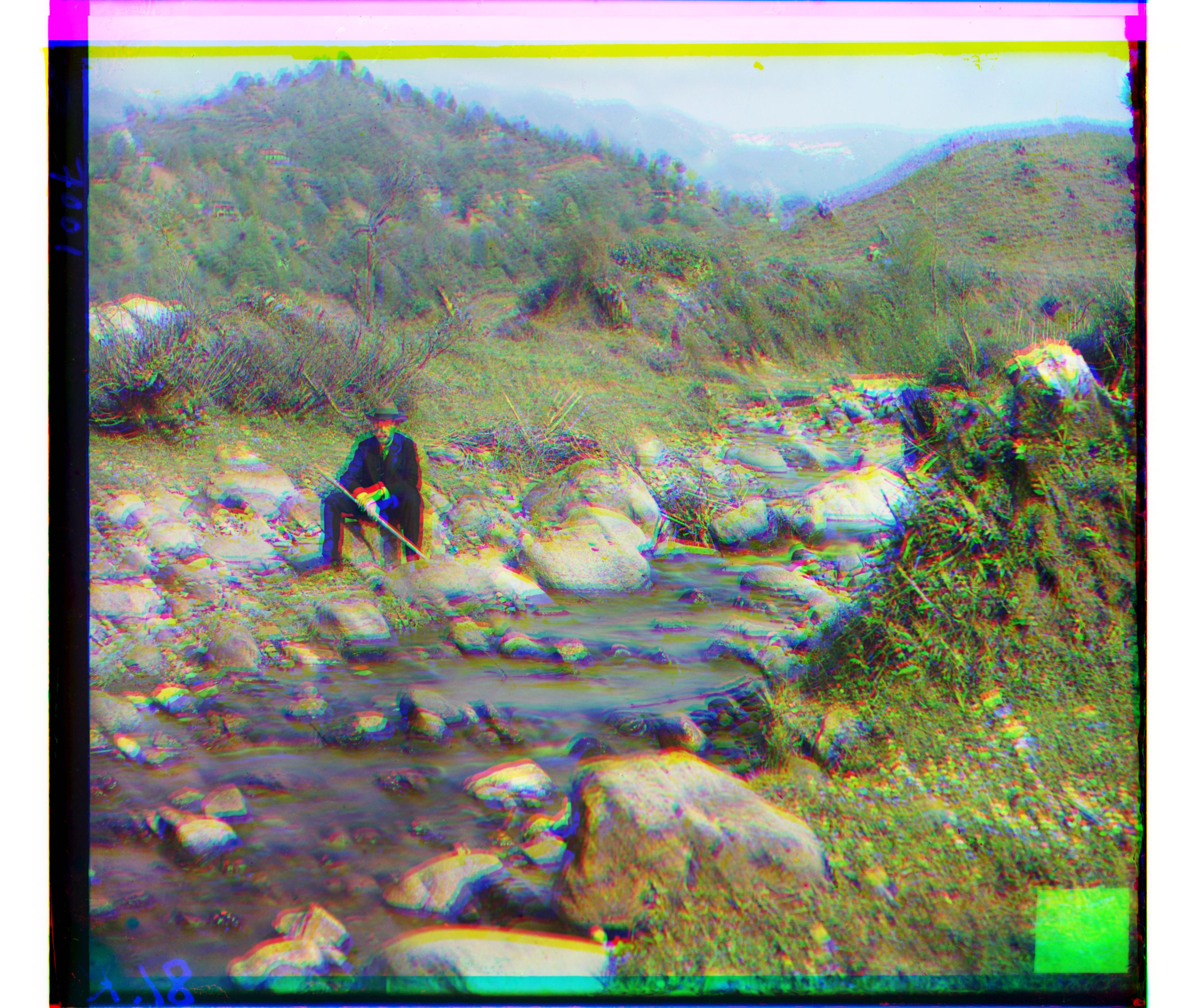
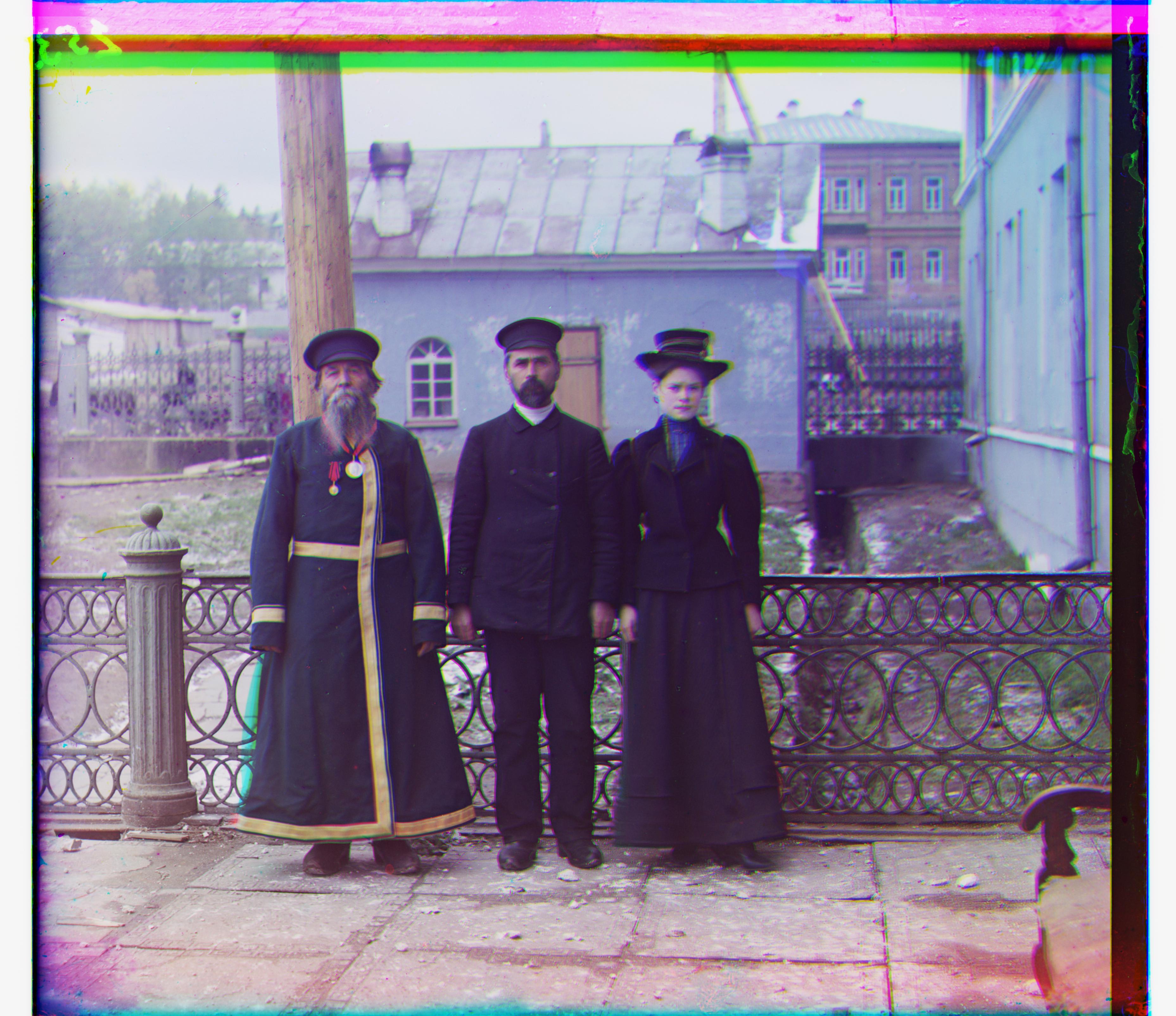
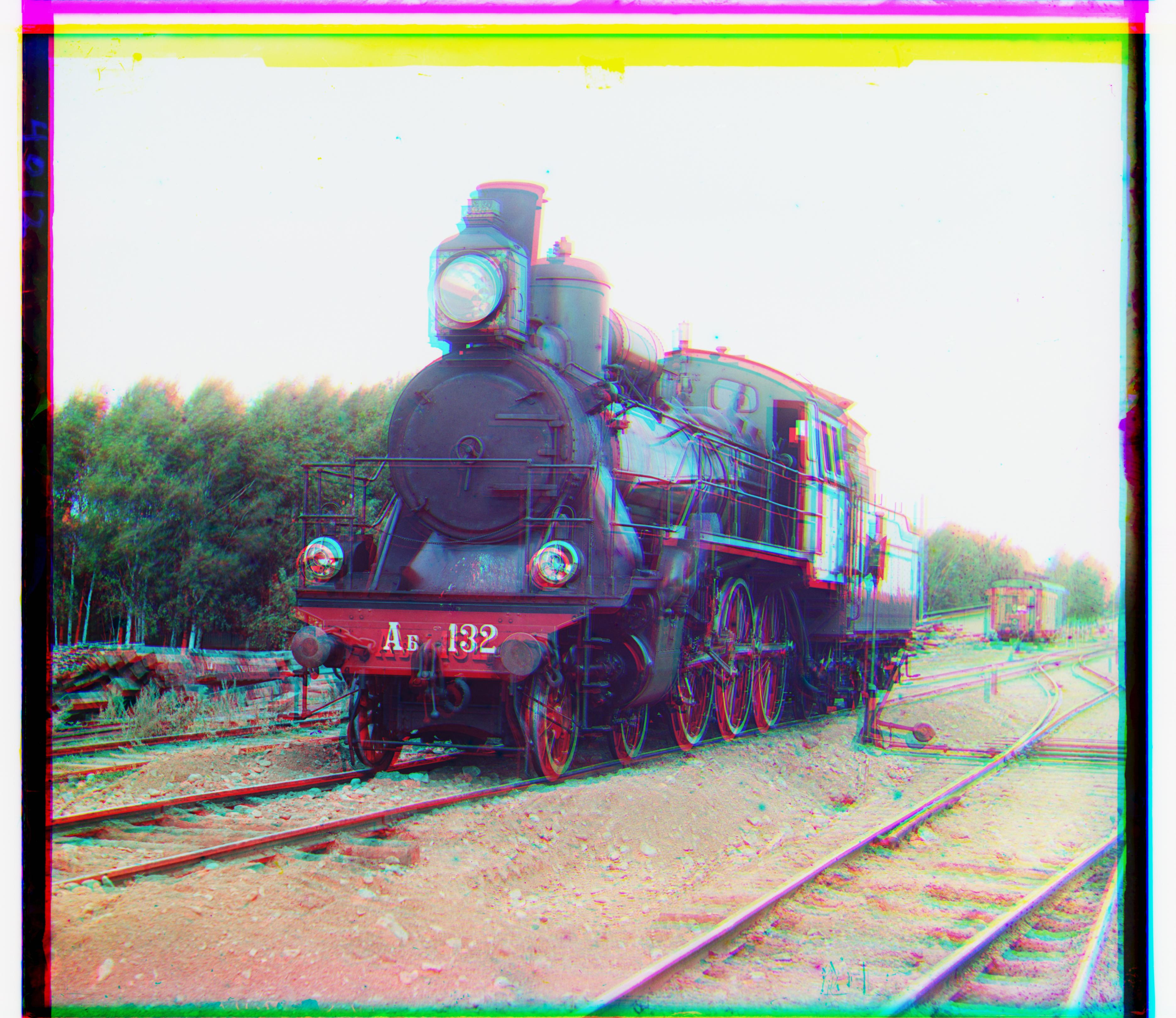
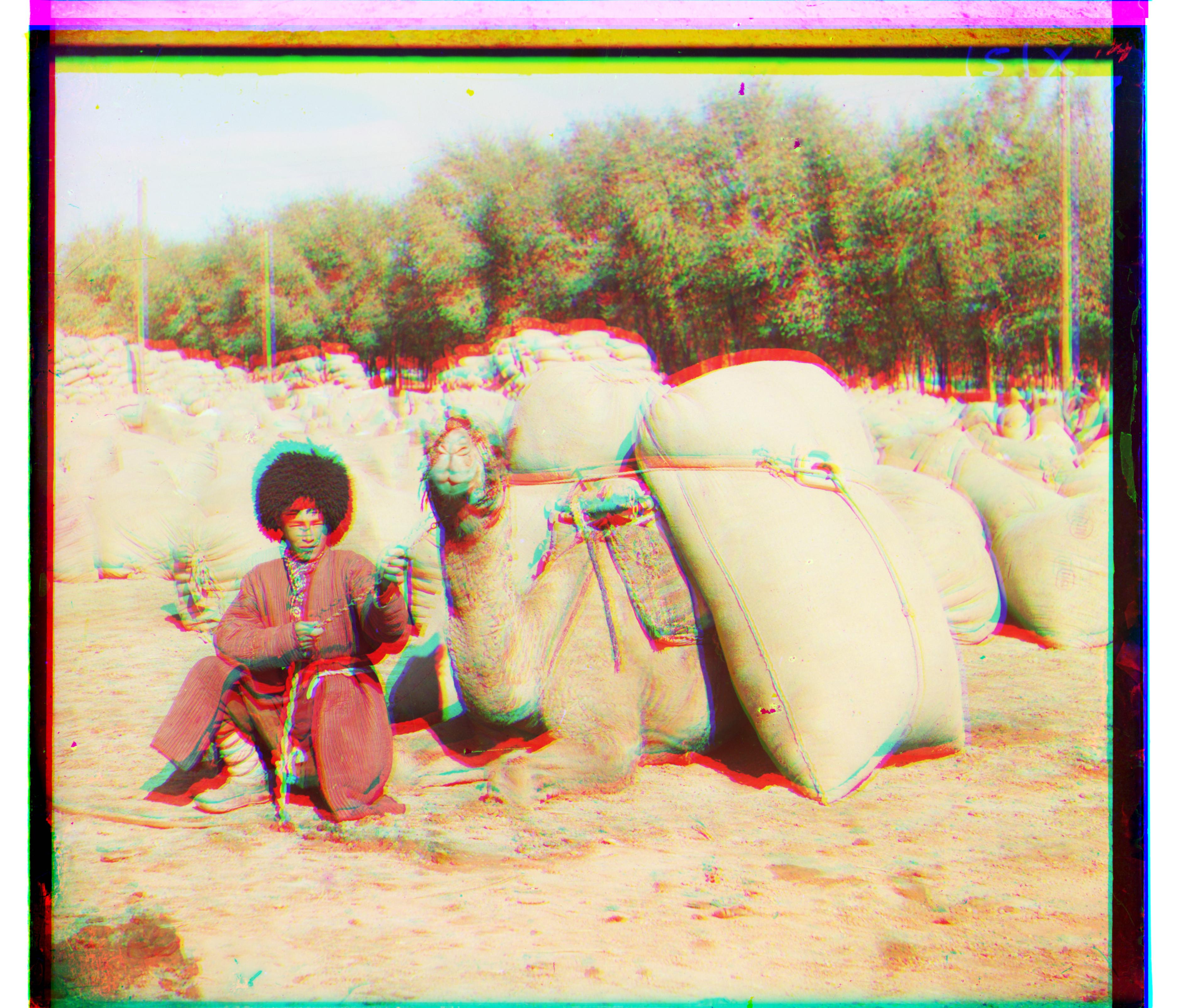
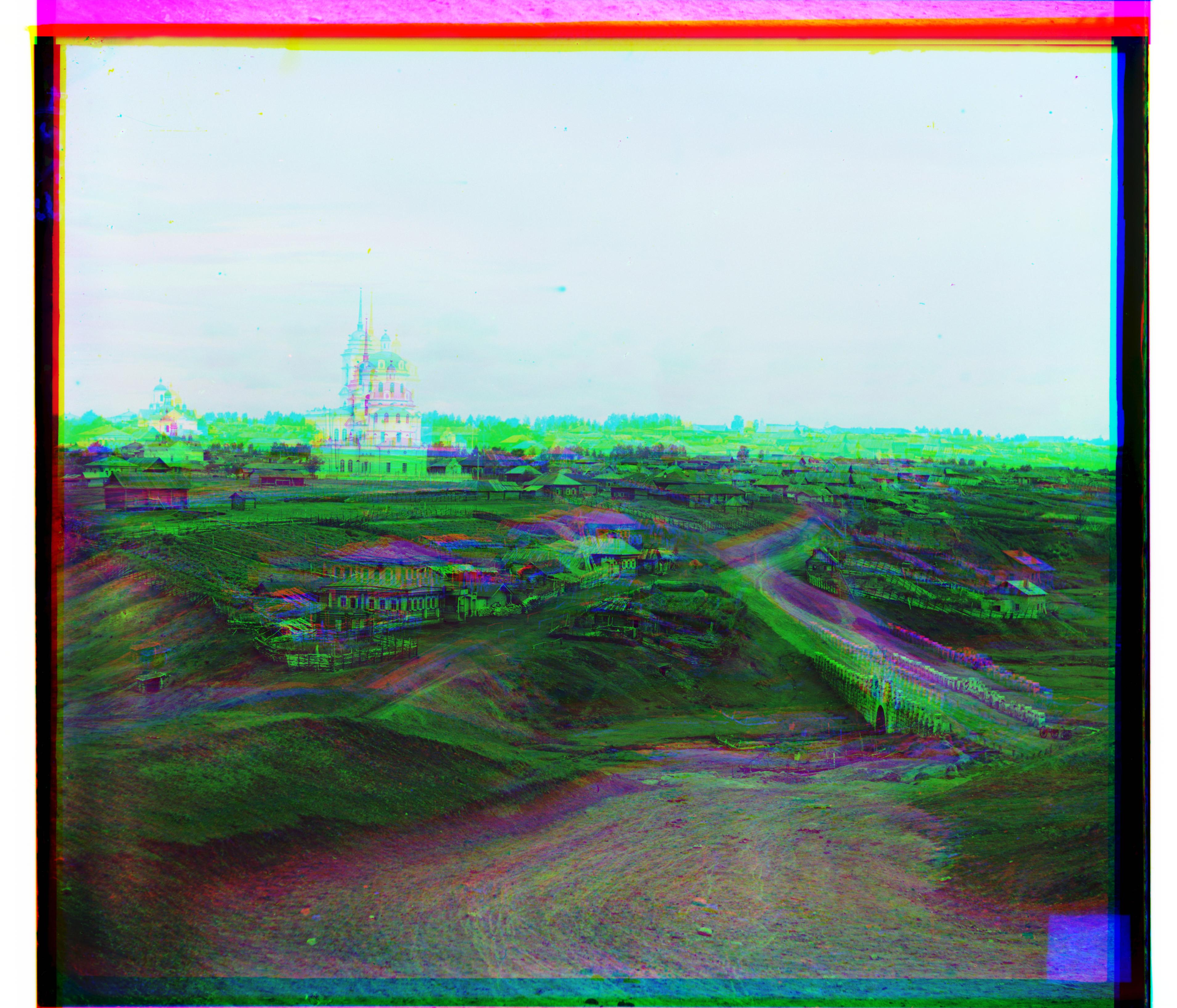
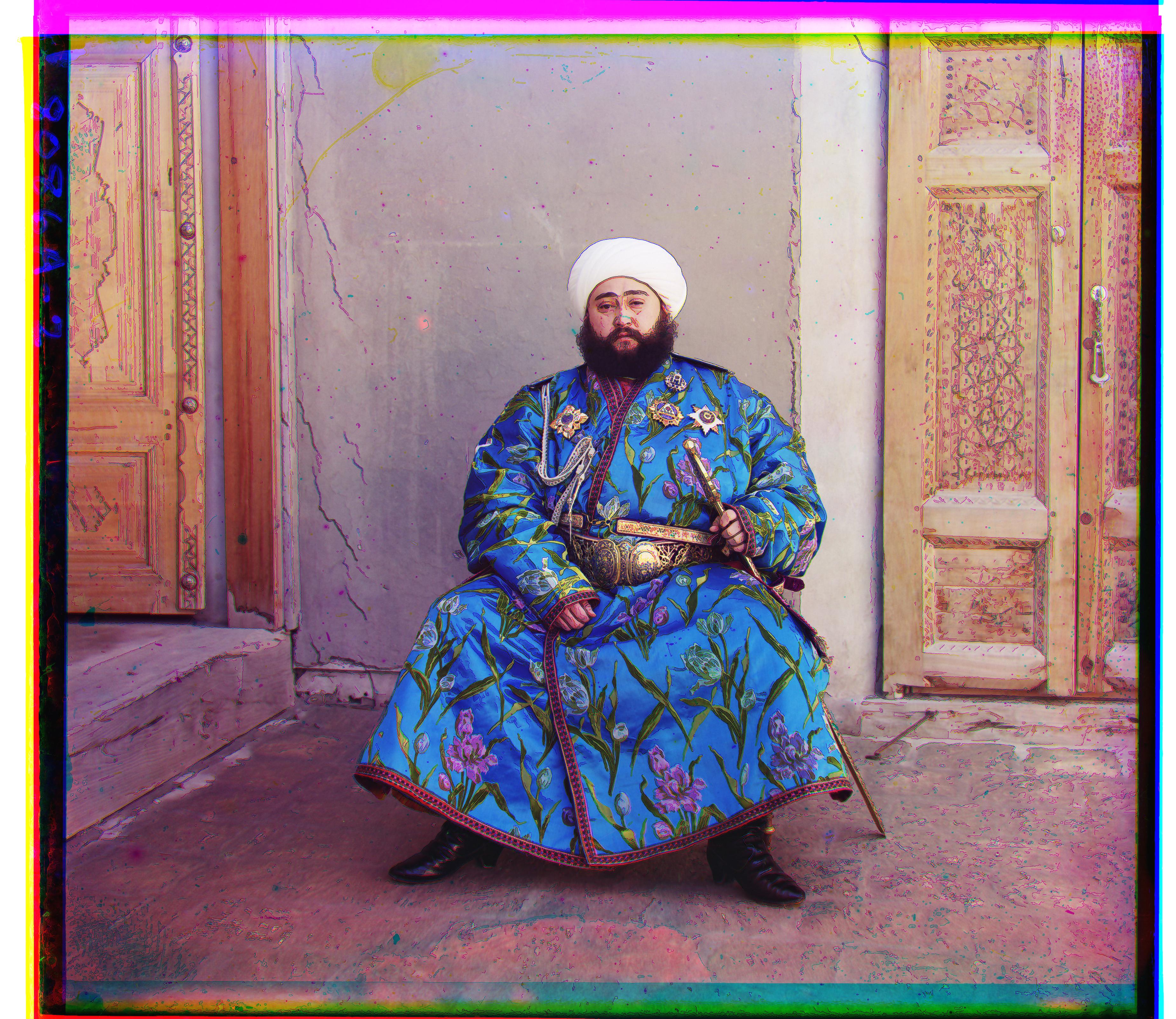
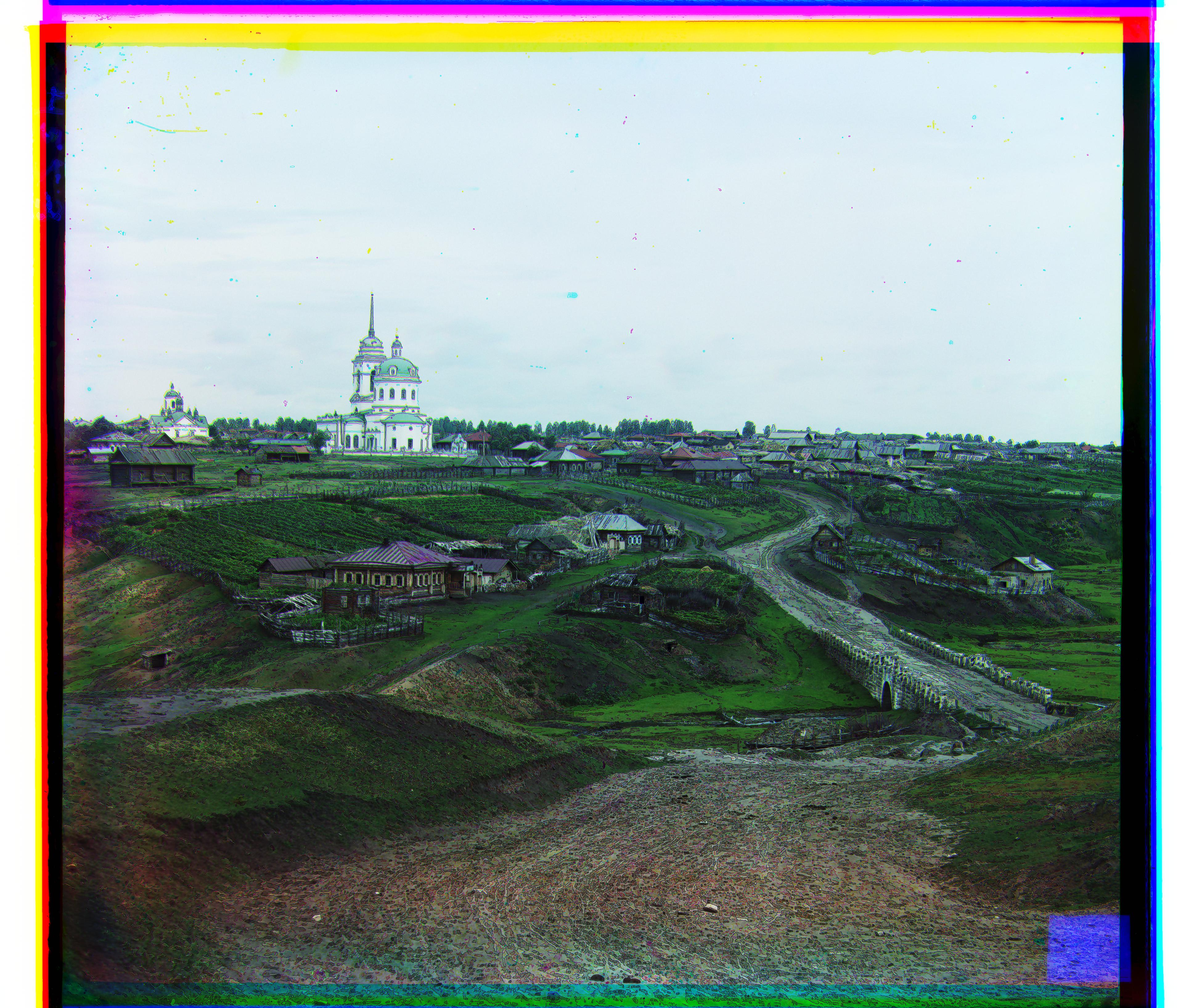
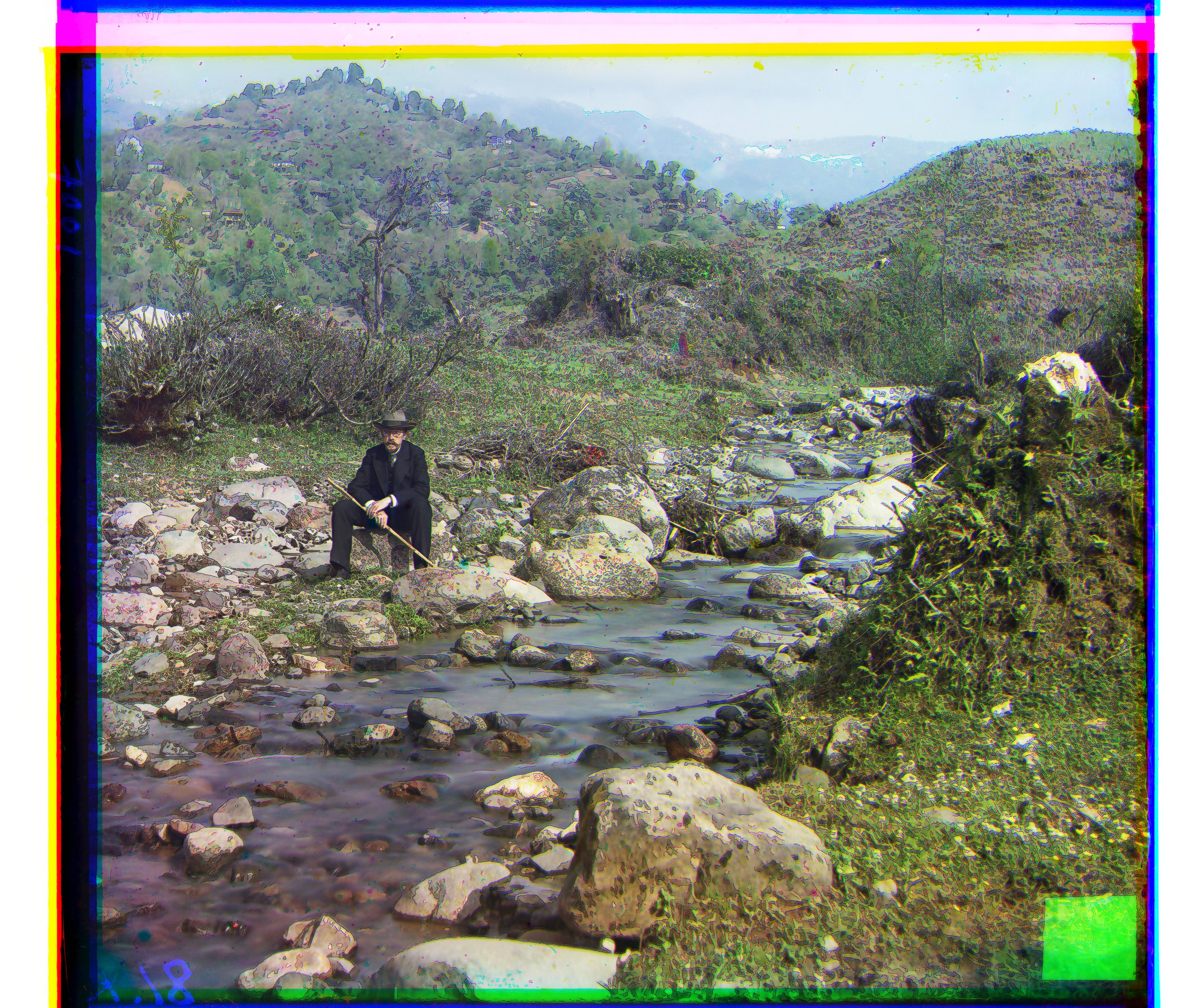
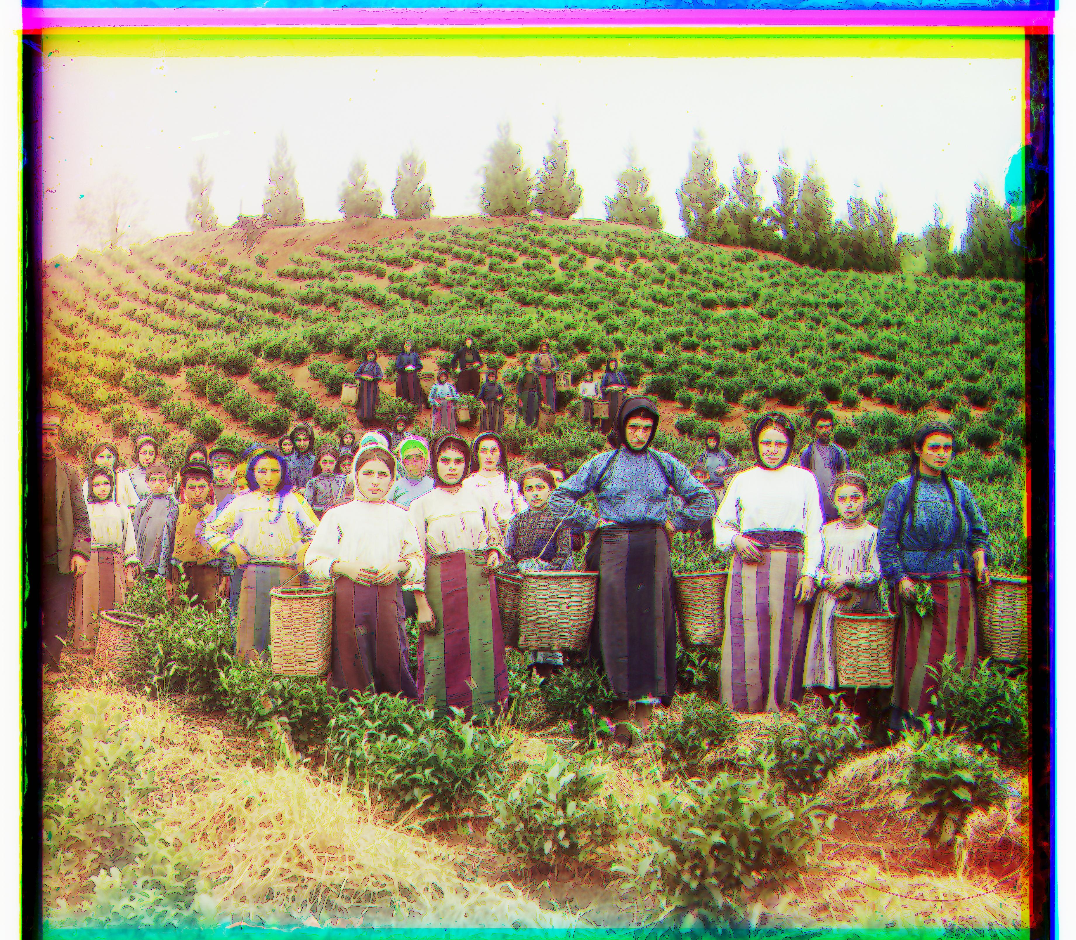
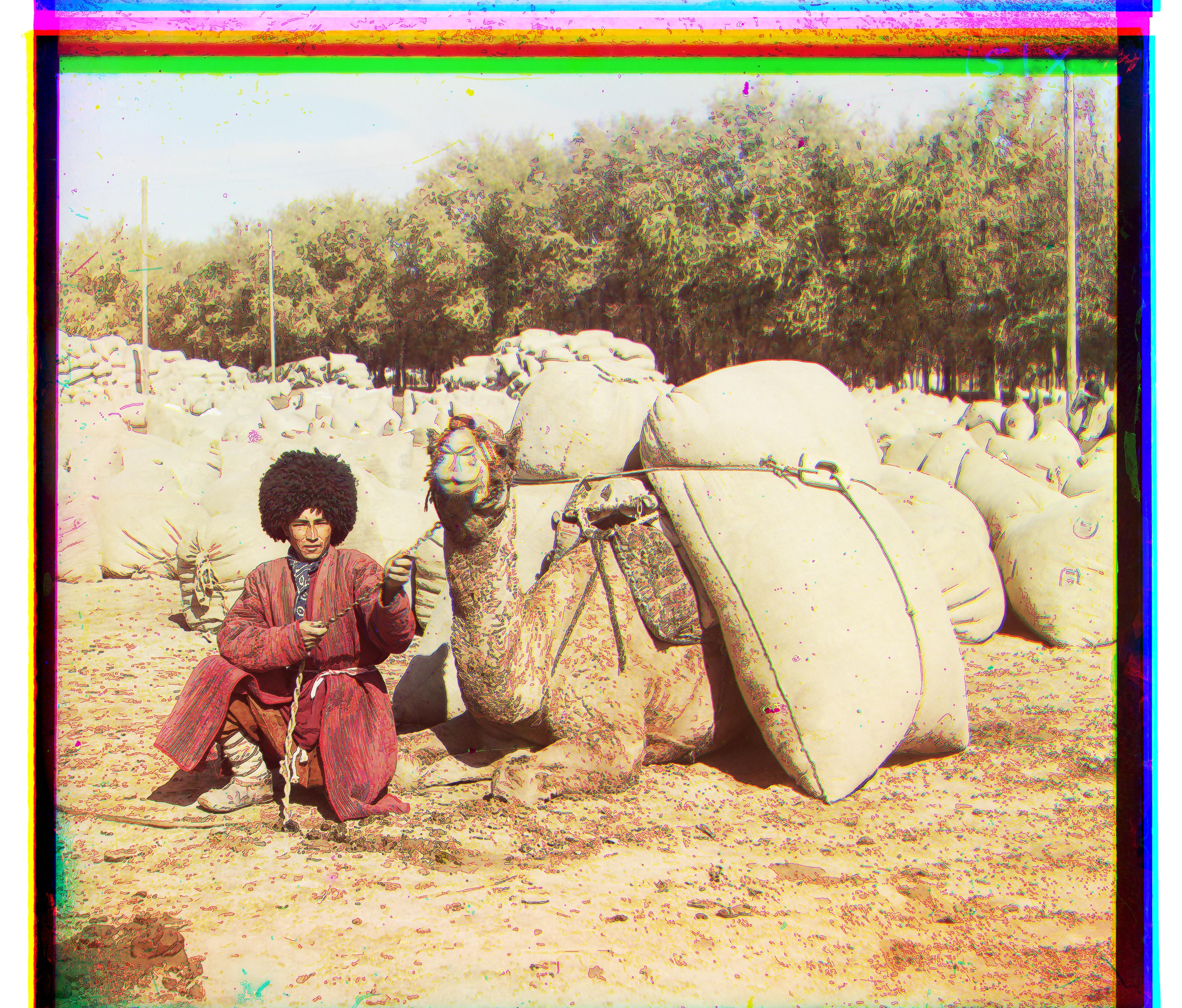
As one can see, some of the photos are slightly blurry. To fix this, the canny edge operator was pre-applied to the red, green, and blue channels. The result was then subtracted from the original channels. The same algorithms were applied. As one can see, the quality of the images improved tremendously. Because a better quality photo was found, a more optimal displacement was found. If you look at the previous pictures, you can see some blurring across the edges of people, objects, and buildings. This probably stems from strong edges in the different channels. Thus, by filtering those channels first, we make the images much clearer. Lady and Icon did not change much after the filtering. This may stem from the fact there were not as many edges/objects in those pictures.
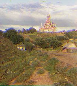
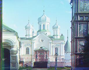
Due to displacements, the images are unfortunately left with some unappealing borders. The standard deviations of three channels across the rows and the columns were calculated. If these standard deviations were below a threshold (0.2) they were removed. If the standard deviation was low across any of the three channels, there was low variance of pixels across that row or column. This was synonymous with there being a border because pixels across the column or row would be the same coloring. This algorithm was run within 15% from the edges of these pictures. Results can be seen below. Perhaps cropping can be improved by increasing the search window from 15% to a larger percentage.
There are several ways to produce auto-contrasting. One of them is through a process called histogram equalizing. It is the process in which the original image is transformed by using a normalized cumalative sum. These old intensity values are mapped to new intensity values so that there is a uniform histogram of intensity values. Another process is contrast stretching. This is the process in which the range of intensity values is stretched. Because a linear scaling function is applied to the intensities, it differs from strict histogram normalization.