Overview
Background
There is no known replica or illustration of the camera that Prokudin-Gorskii used. It was a view camera of his own design, perhaps similar to a model designed about 1906 by Dr. Adolf Miethe, whom Prokudin-Gorskii had met previously in Germany.
We know that Prokudin-Gorskii intended his photographic images to be viewed in color because he developed an ingenious photographic technique in order for these images to be captured in black and white on glass plate negatives, using red, green and blue filters. He then presented these images in color in slide lectures using a light-projection system involving the same three filters.
Naive Approach
SSD(sum of squared differences)
I began the project using a simple and straightforward algorithm called SSD (sum of squared differences) which performed an exhaustive search of all possible alignment offsets of one image compared to another in the interval [-15, 15] and picked the one that has the maximum value after multiplication. The maximum value means the two images are aligned together in the most fittable way. After computing the best offset for the r and g channels along with r and b channel, the three channels ultimately aligned the best way.
Second Approach
Gaussian Pyramid Algorithm
The small interval window of [-15, 15] is sufficient for small images with a width of under 300px. However, if the image resolution is large, the offset window might not be sufficient for finding the correct offset. Besides, computing the SSD of large images multiple times is time consuming and not efficient. Because of these reasons, we apply a Gaussian pyramid method for shrinking images.
The concept of Gaussian pyramid is first applying a Gaussian blur on the image with a small window (3-by-3 or 5-by-5). The blurred image is then downsampled into a new image of half the width and height. Due to blurring, the major details of the images are preserved.
Gaussian pyramid is applied multiple times (layers) on the image until the result has a width of less than 300px. Then we can use the small interval window in a efficient way and calculate the offset of the small images. After obtaining these offsets, the total offset is acquired by multiplying the small offset with 2 to the nth power, where n is the number of layers of the Gaussian pyramid used.
Before Auto Cropping
After Auto Cropping
Auto Cropping
At first, I began crop my image using cut off 0.1 of the left, right, up and down side. However, this is not detecting any borders. Then, I used the RG and RB offset to crop the non-overlapping parts out.
Auto Contrasting
Auto Contrasting
The auto-contrasting procedure re-scales the luminance range of the entire image to [0,1]. In order to achieve this, the function first needs to find the pixel with highest luminance value. Because of that, the RGB image is converted into grayscale and the highest grayscale value is considered the largest luminance. Working under the assumption that luminance is evenly distributed between all three channels, the scaling factors of each channel simply becomes the inverse RGB values of the pixel with highest grayscale value. These scaling factors are then applied across the entire image and the result is an auto-scaled image with luminance of [0,1].
Before White Balancing
After White Balancing
White Balancing
The Gray World Assumption is a white balance method that assumes that your scene, on average, is a neutral gray. Gray World assumes that all the colors in an image ought to average out to a neutral gray: for every blue there is a yellow, for every red there is a cyan, and for all greens there are magentas. In this project, I adjust the curves until all the RGB values are equal
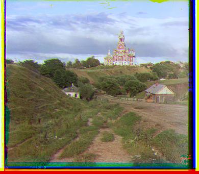
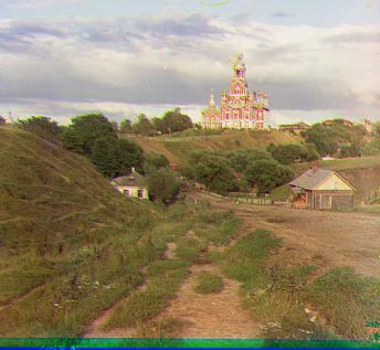
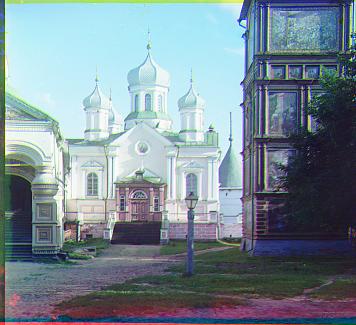
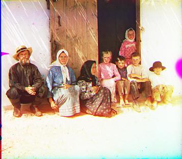
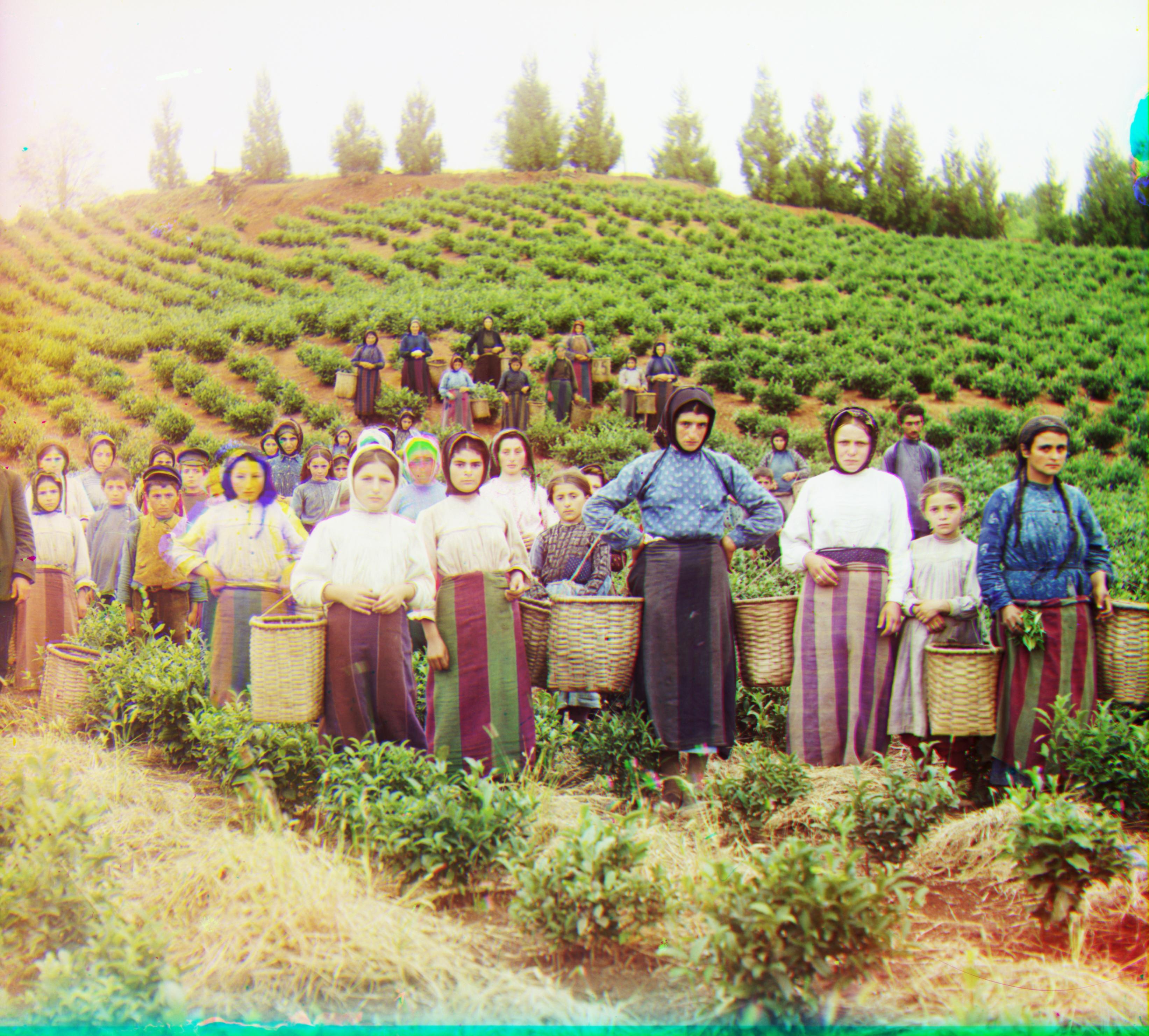
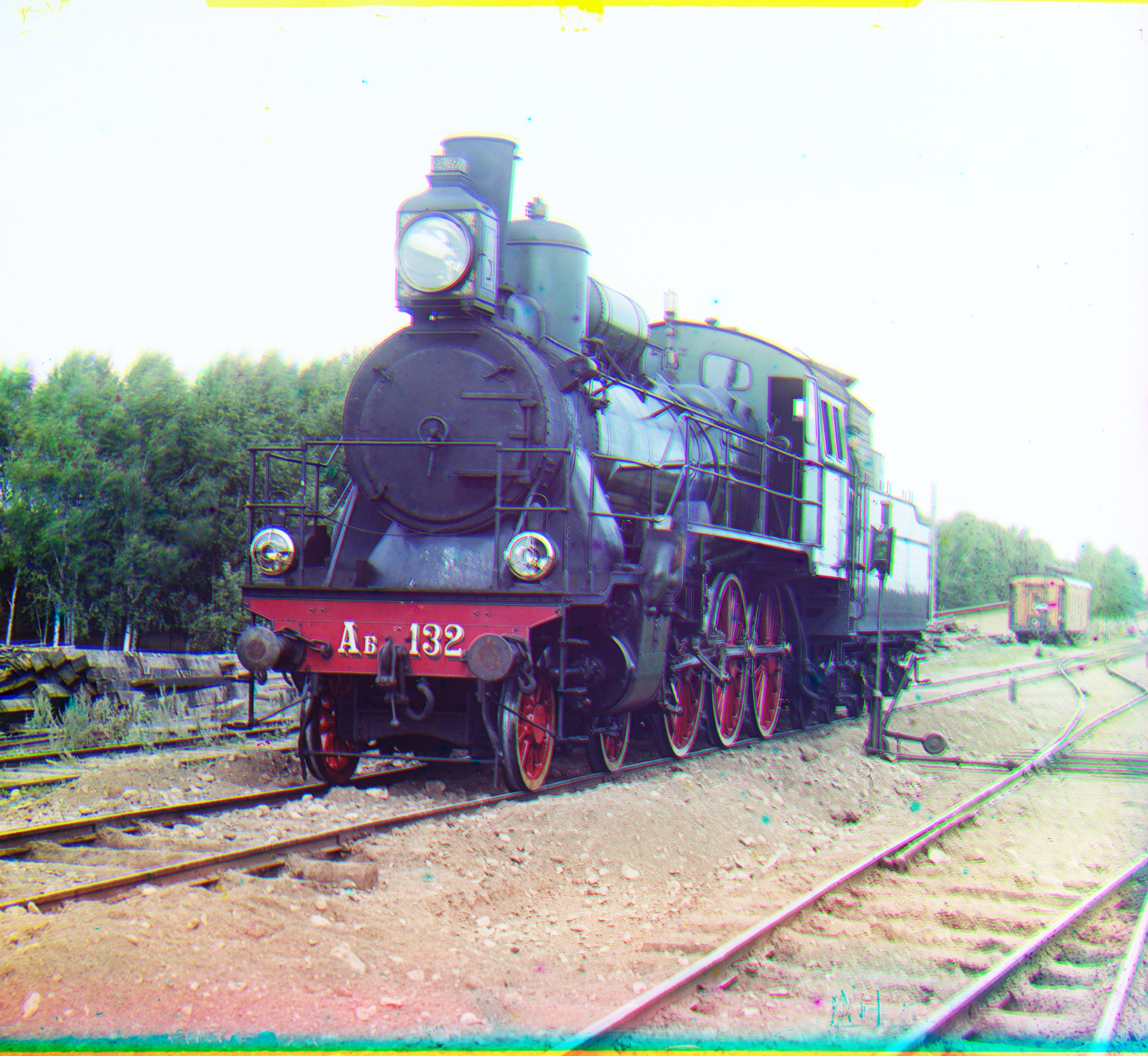
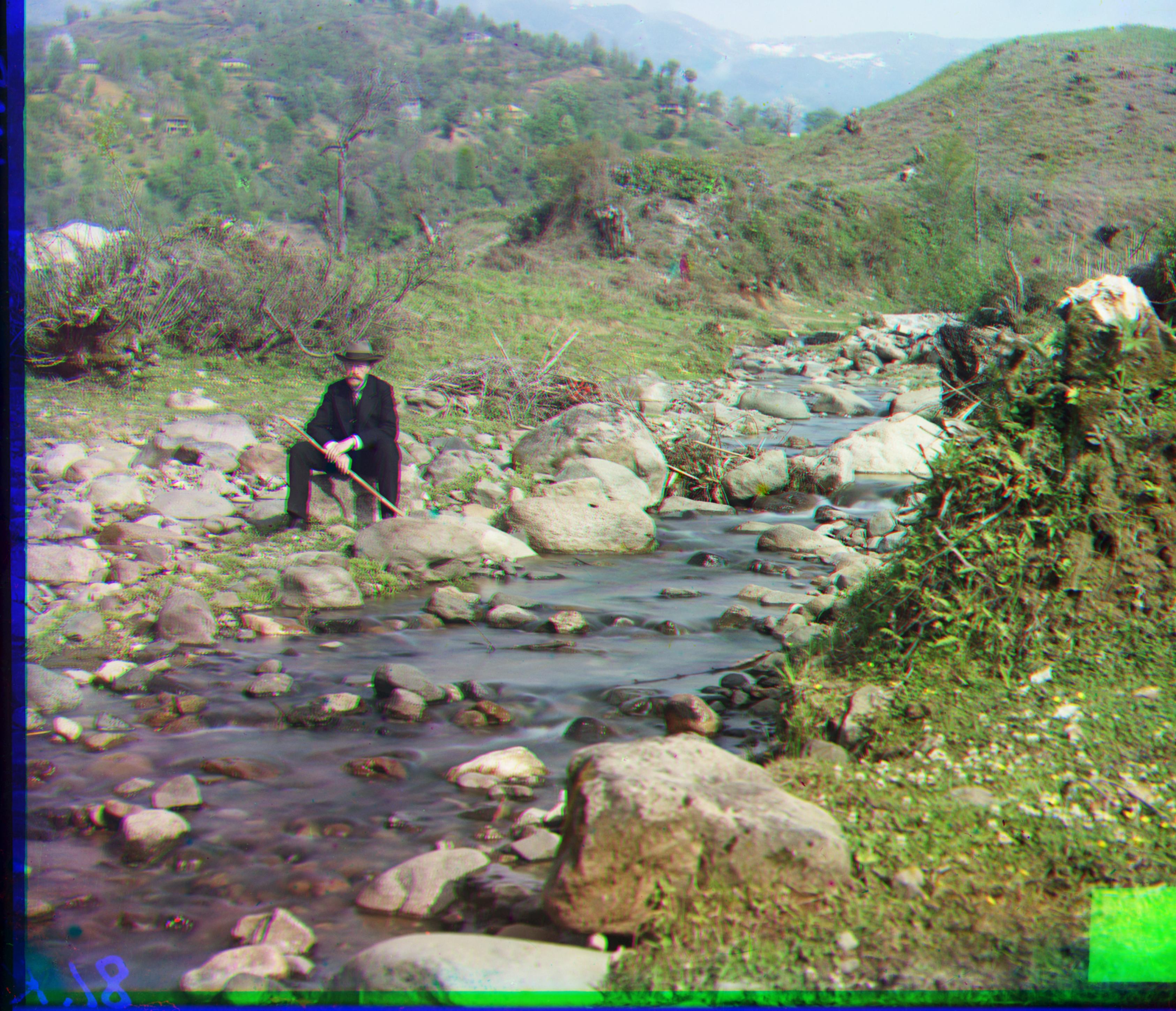
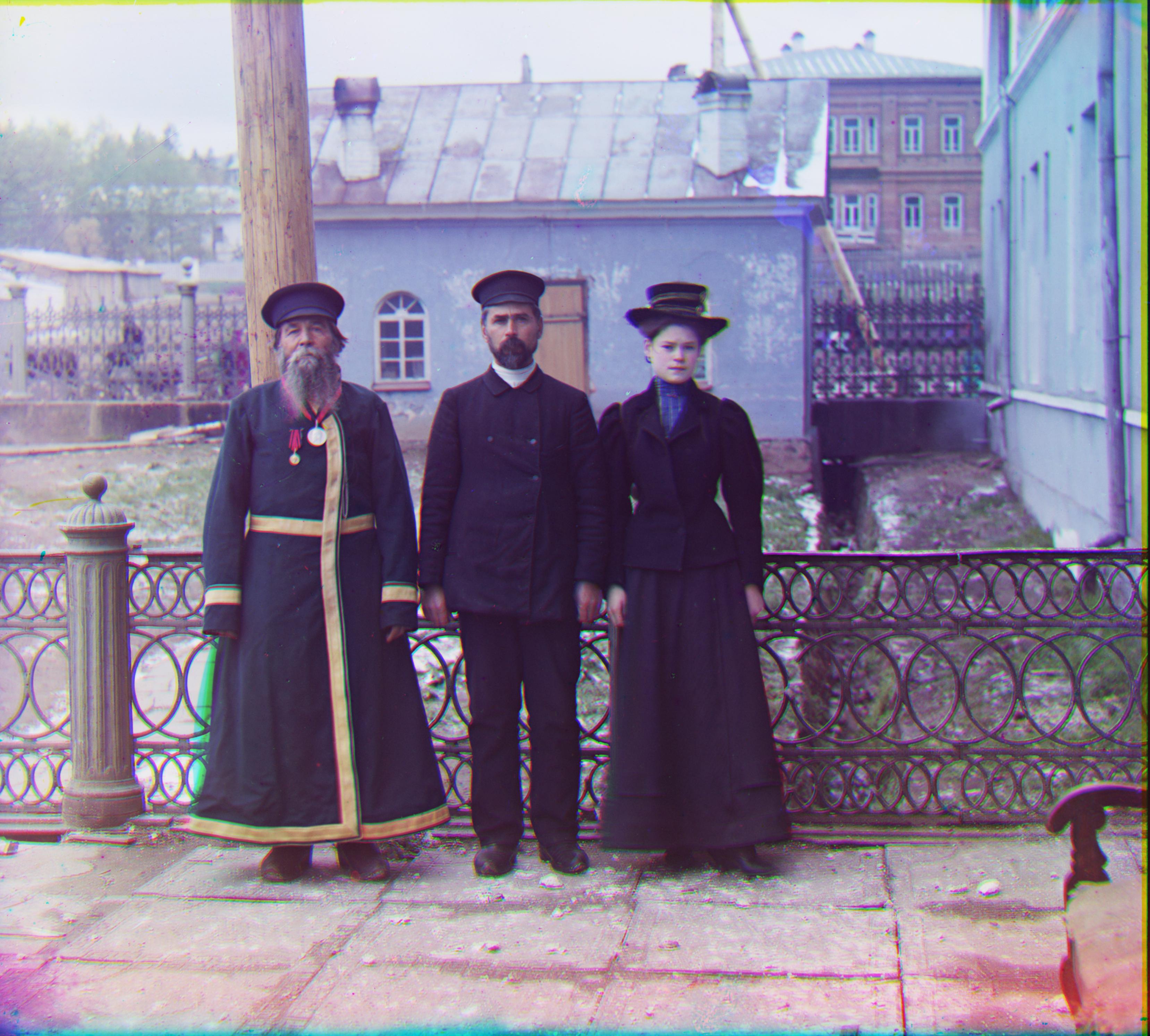
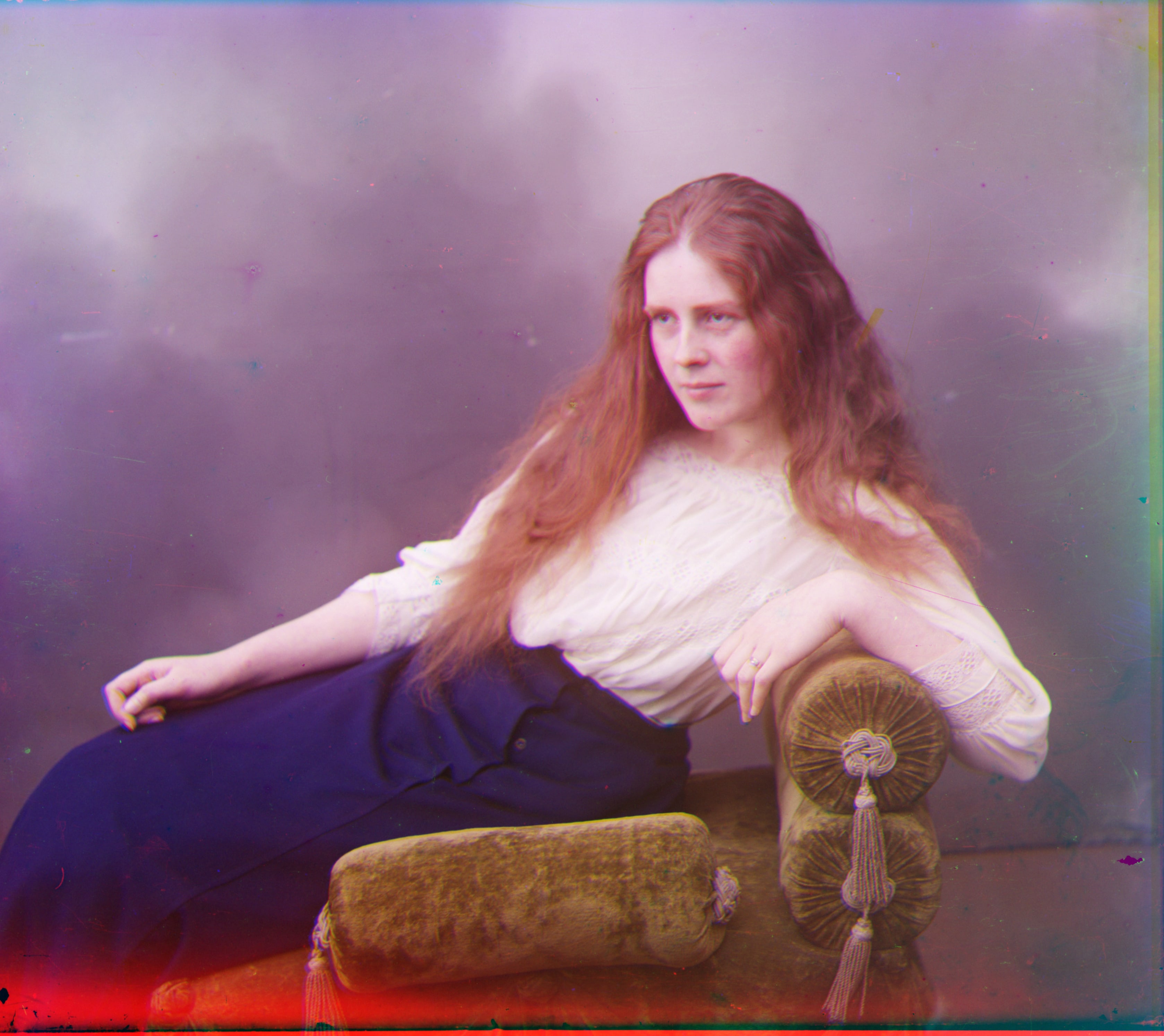
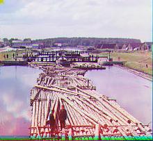
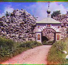
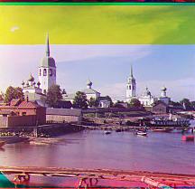
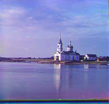
Examples given by project 1
1.215414s RB:[12,4] RG:[6,0]
1.176140s RB:[2,2] RG:[6,0]
1.259833s RB:[8,0] RG:[4,0]
1.249178s RB:[14,0] RG:[8,0]
2.676224s RB:[128,16] RG:[64,0]
2.769171s RB:[96,16] RG:[48,0]
2.883804s RB:[96,32] RG:[48,32]
2.740531s RB:[176,32] RG:[96,0]
2.675022s RB:[112,16] RG:[64,0]
2.795022s RB:[112,32] RG:[64,0]
2.675022s RB:[112,16] RG:[64,0]
2.828304s RB:[112,32] RG:[64,16]]
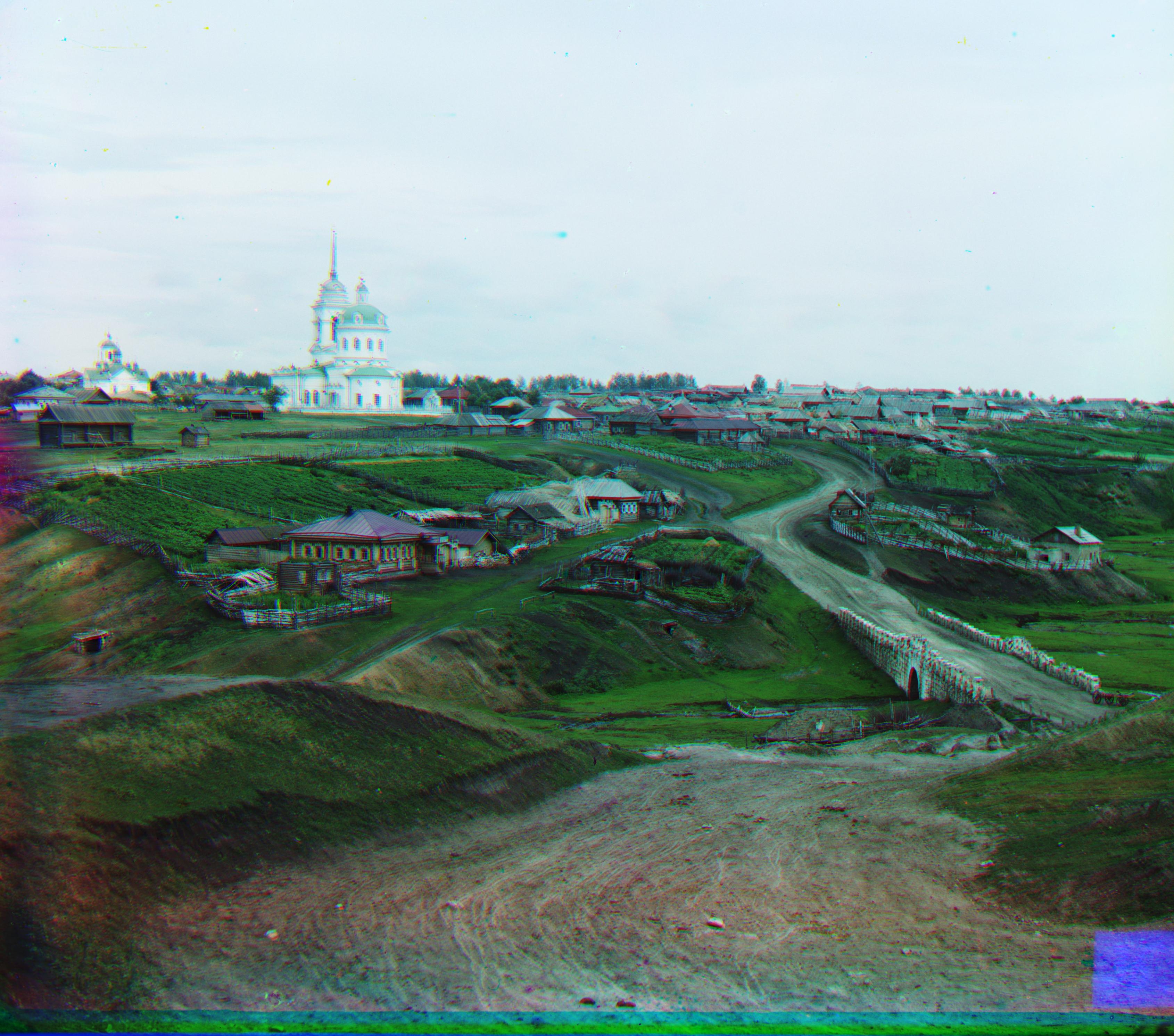
2.866064 RB:[112,16] RG:[64,0]
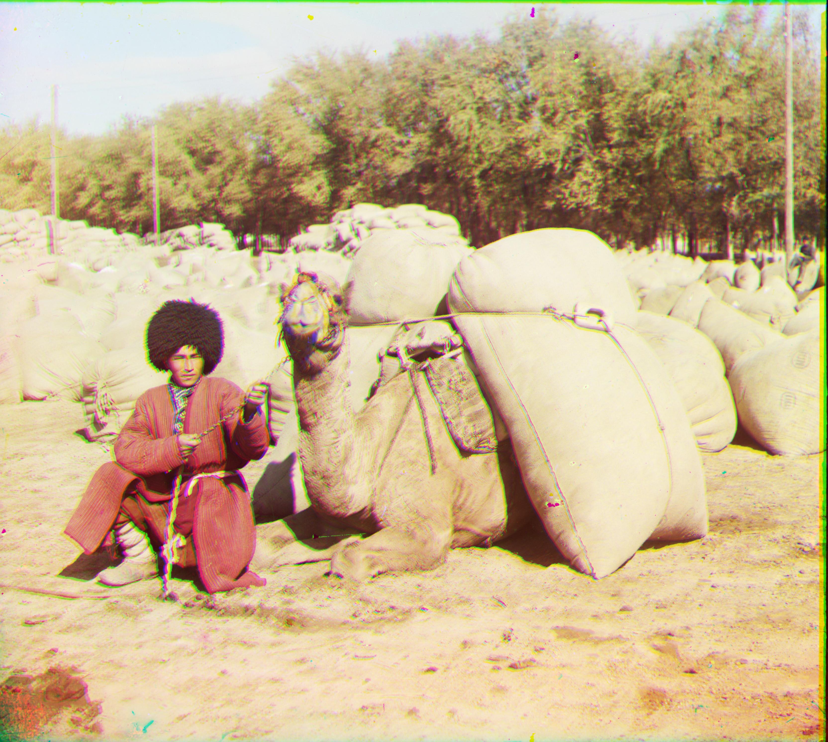
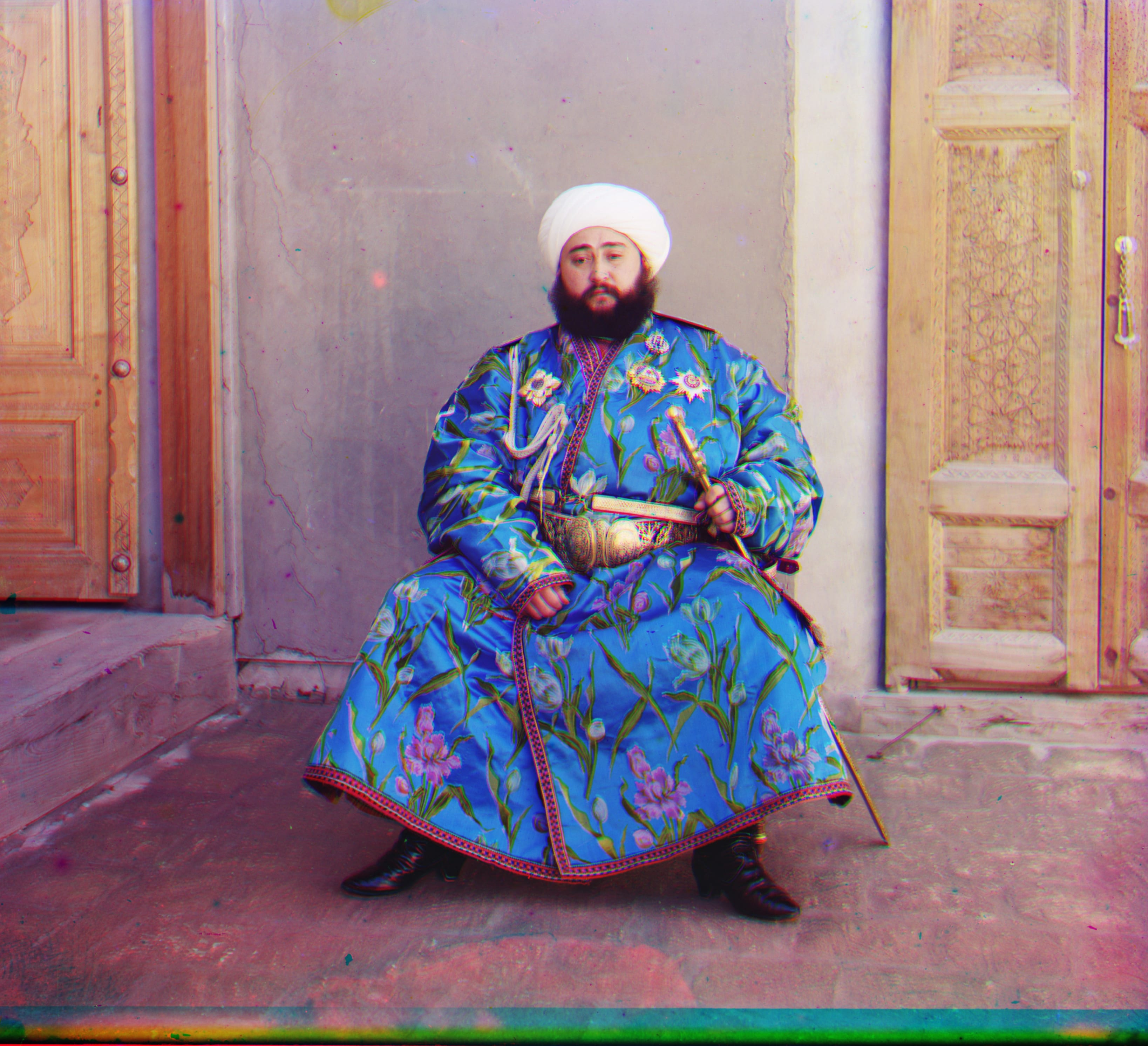
Samples from Ohter website
1.067461s RB:[5,0] RG:[2,0]
1.042318s RB:[2,1] RG:[1,0]
1.021541s RB:[2,2] RG:[1,0]
1.002540s RB:[3,-1] RG:[2,0]