

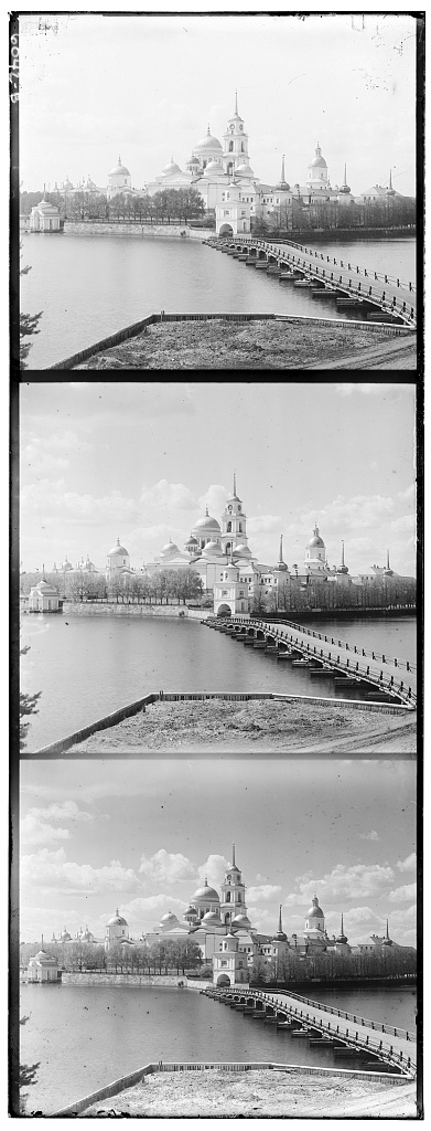
In the early 20th century, Sergei Mikhailovich Prokudin-Gorskii was given permission by the Tzar to travel across the Russian Empire to take color photographs. He was clearly a man ahead of time-- color photography did not yet exist at the time. He recorded three exposures of each scene using red, green, and blue filters. His RGB glass plates were digitized and made available by the Library of Congress. Each set of negatives appears as three separate images, corresponding to the blue, green, and red channels; these must be stacked to produce a color image.
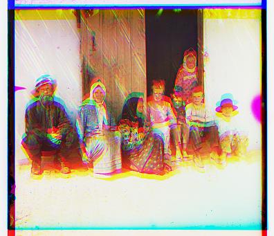
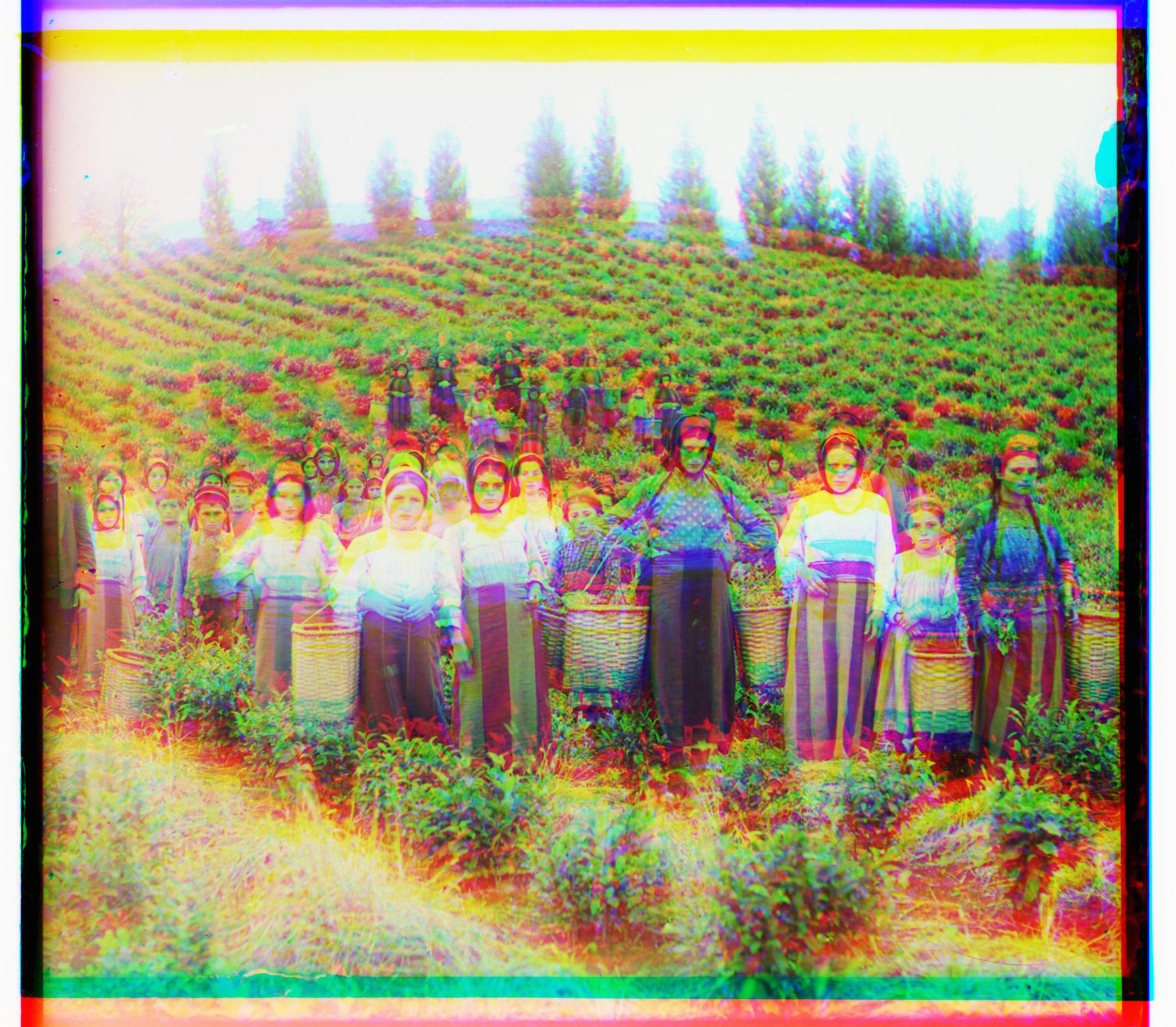
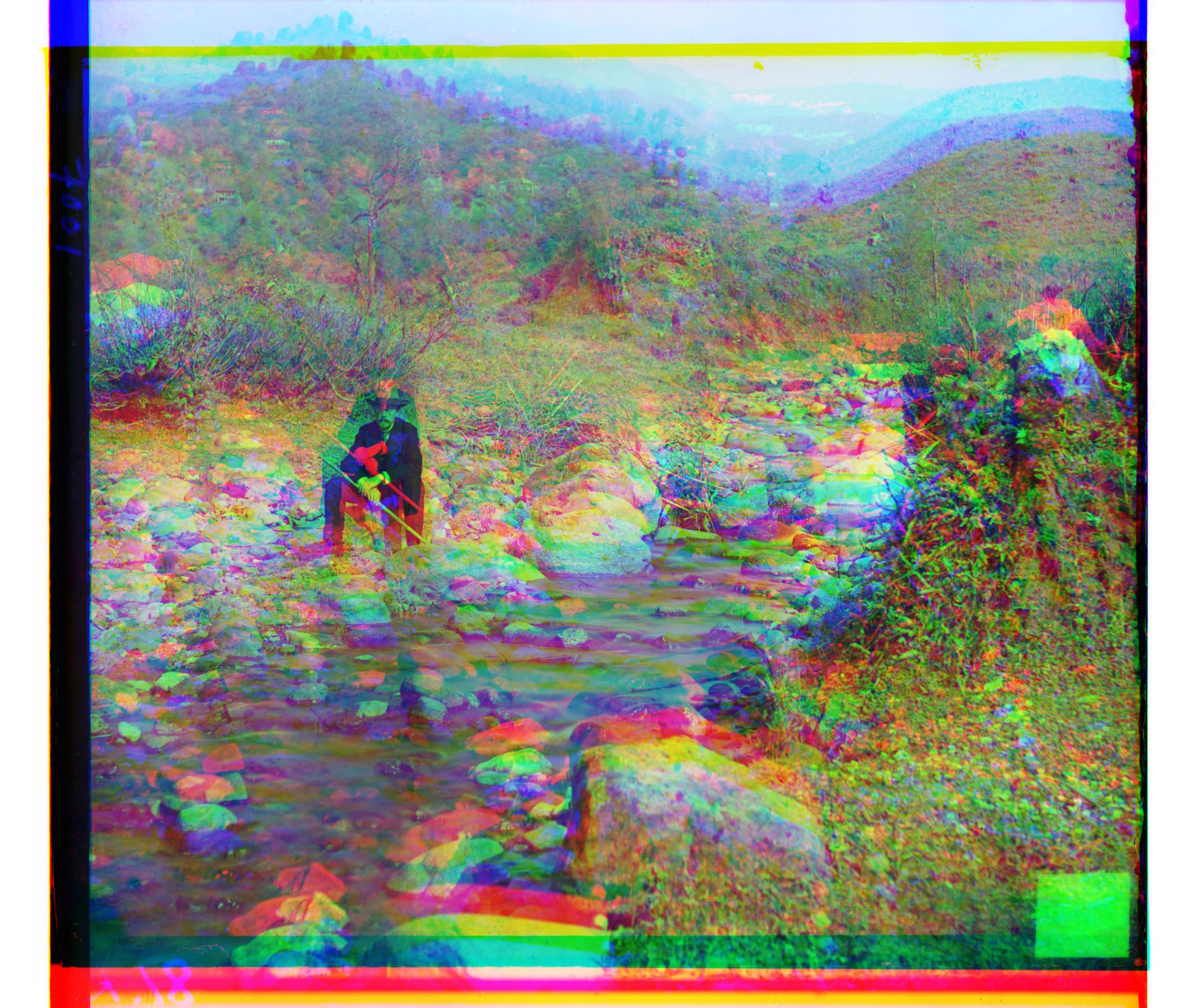
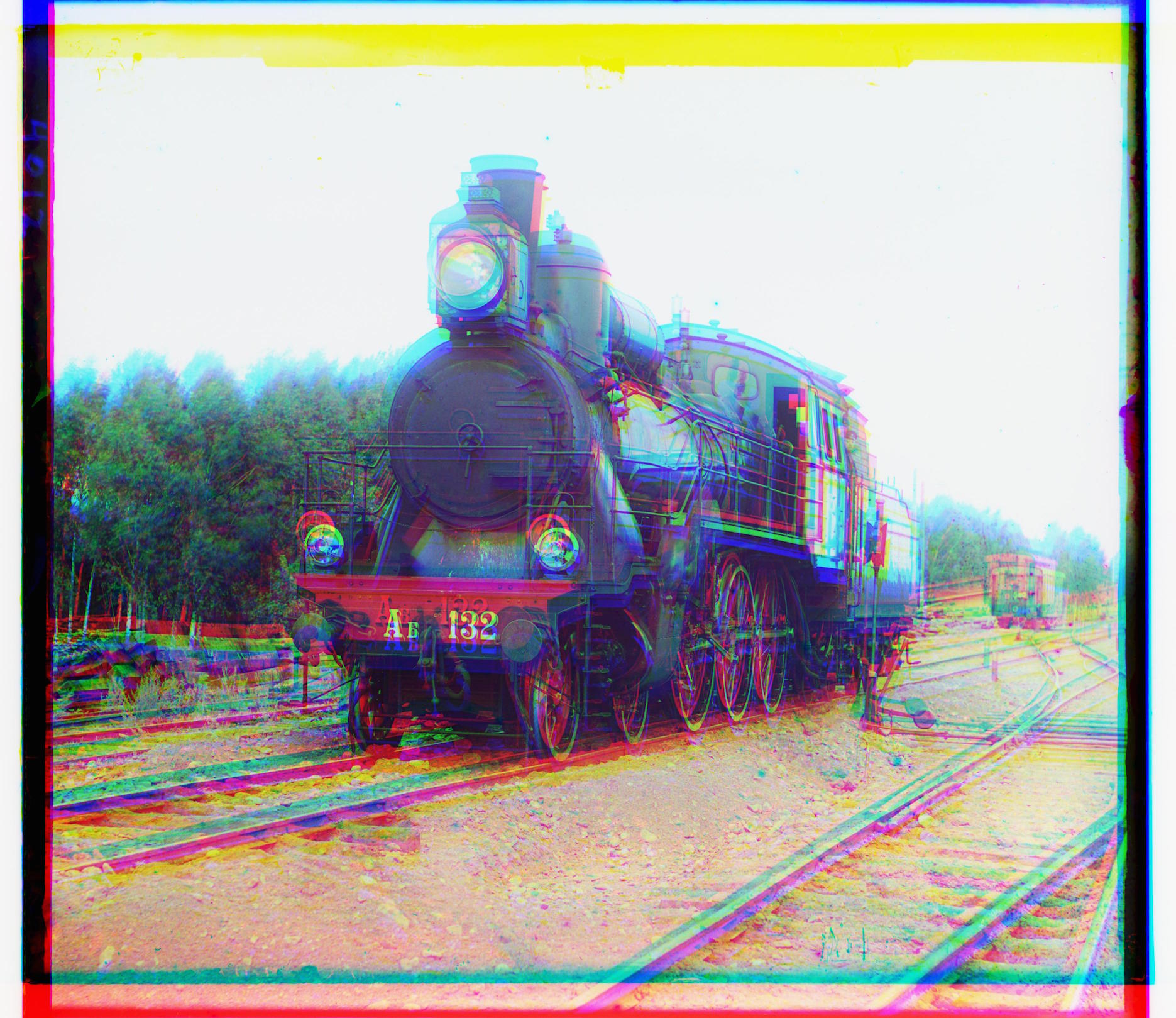
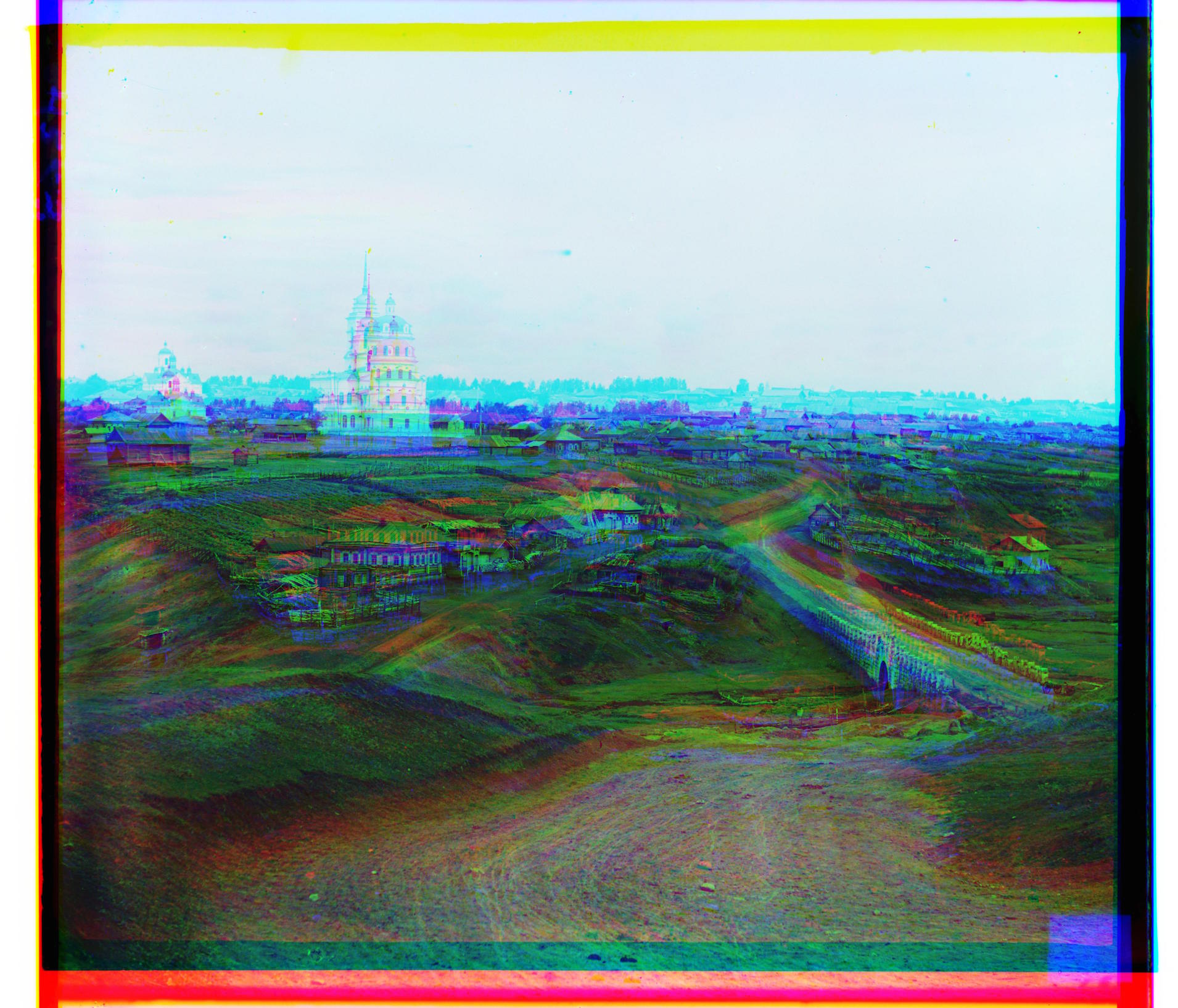
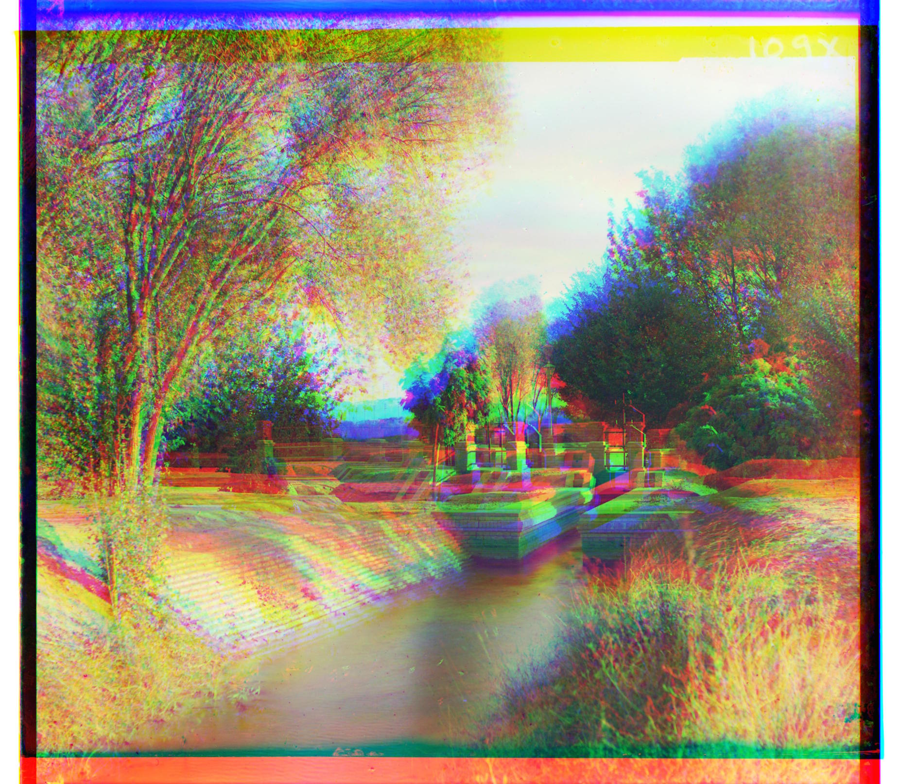
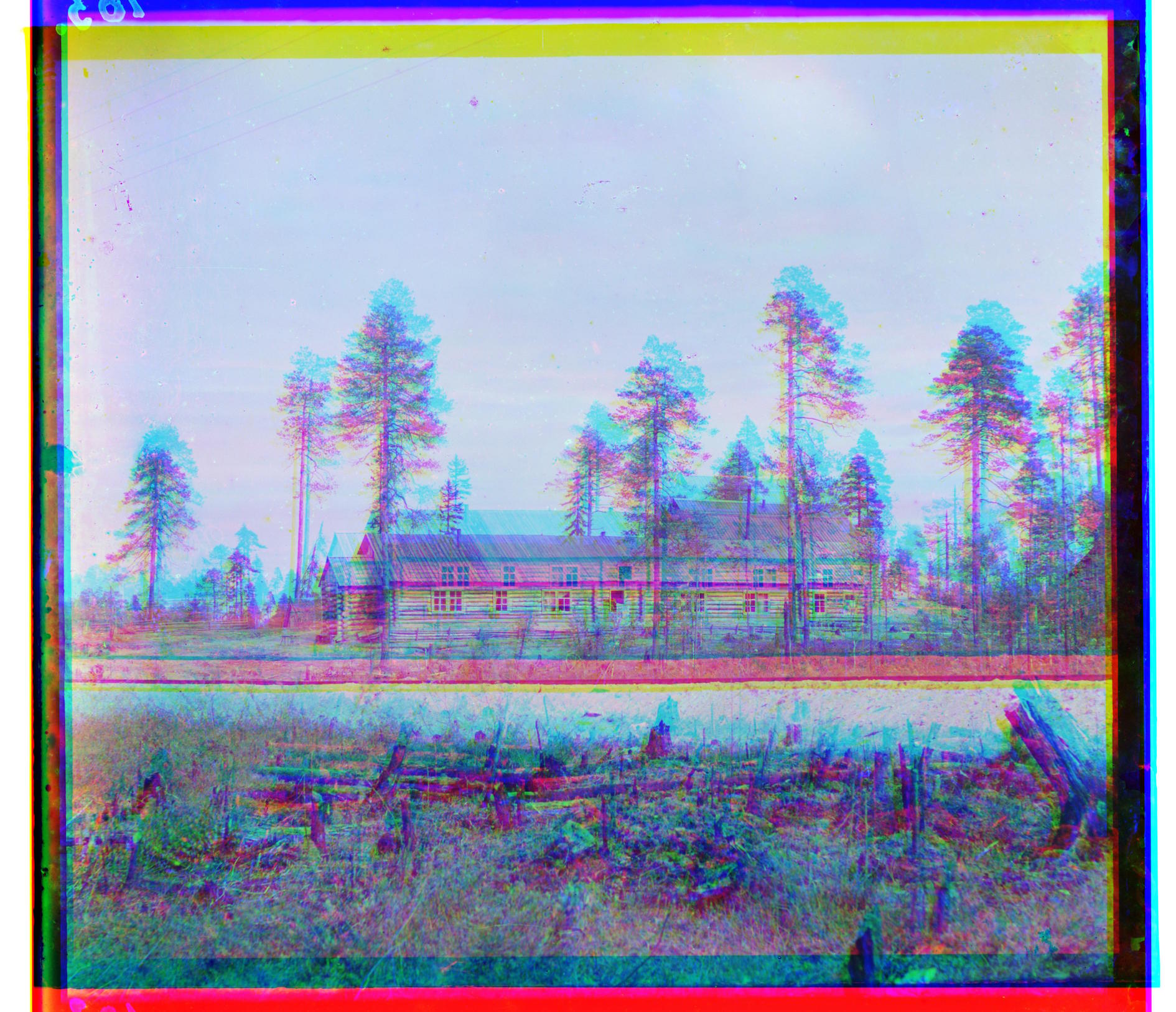
If you just stack the three channels with no effort to align them, you will get a very blurry picture (see the "Before" column below).
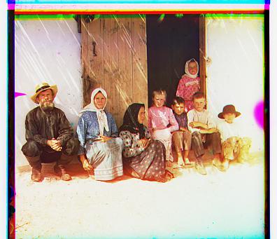
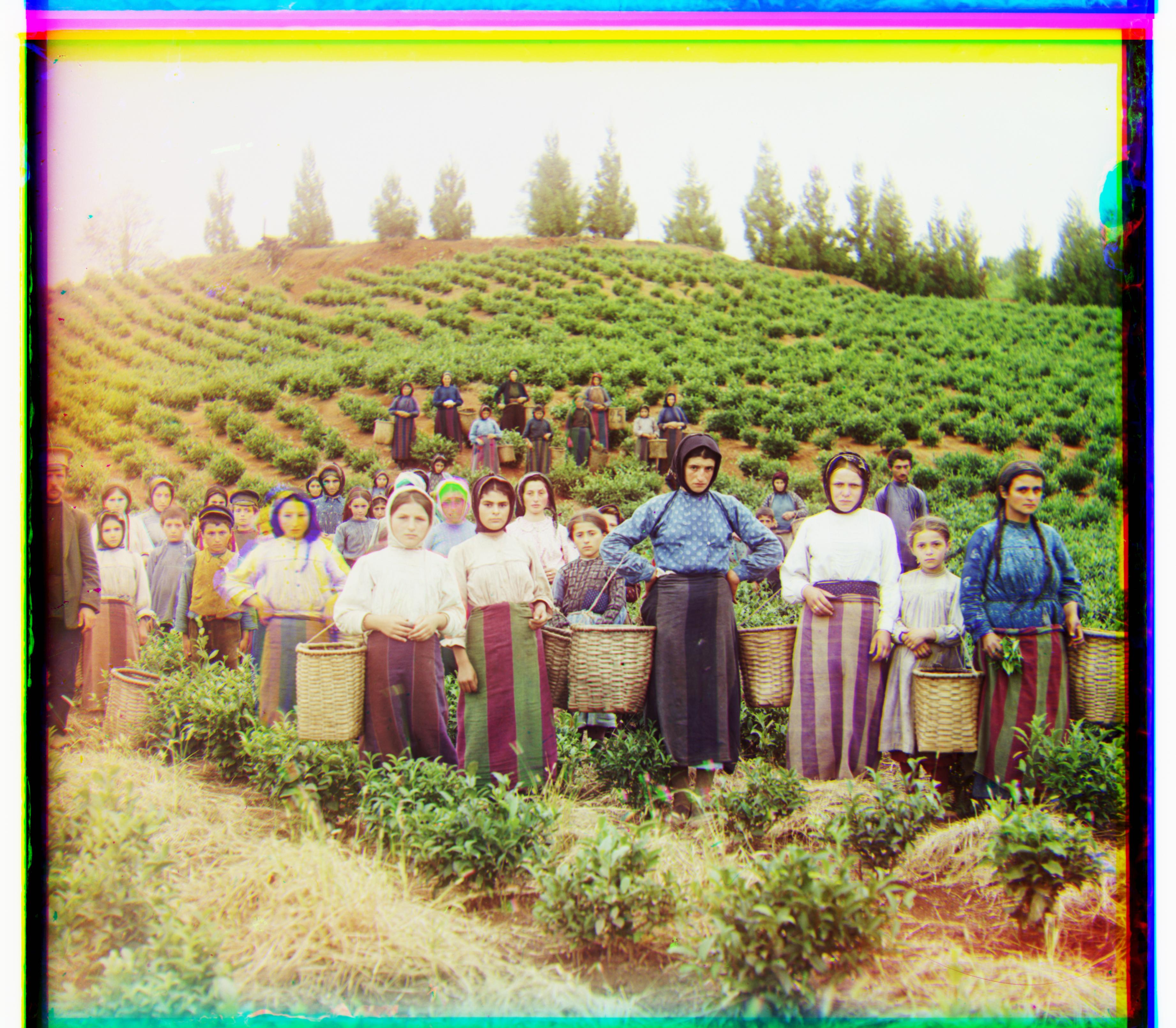
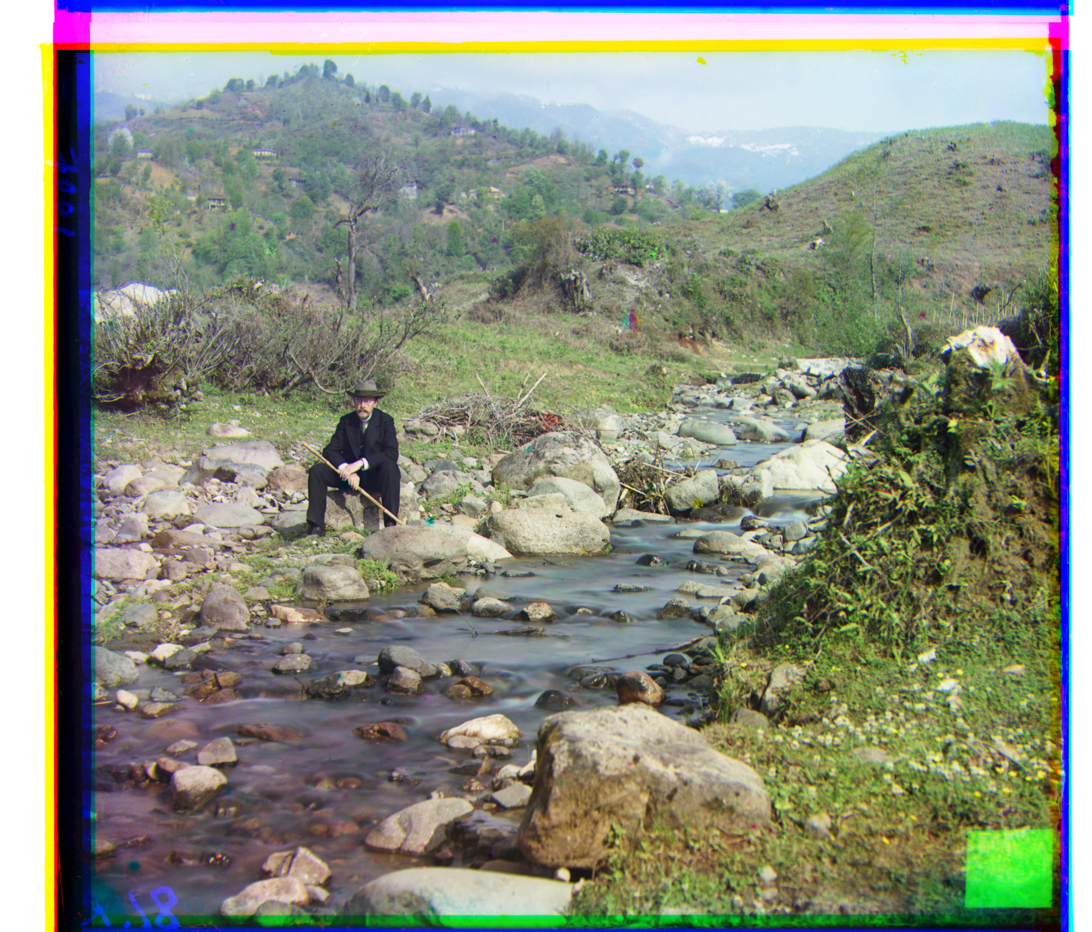
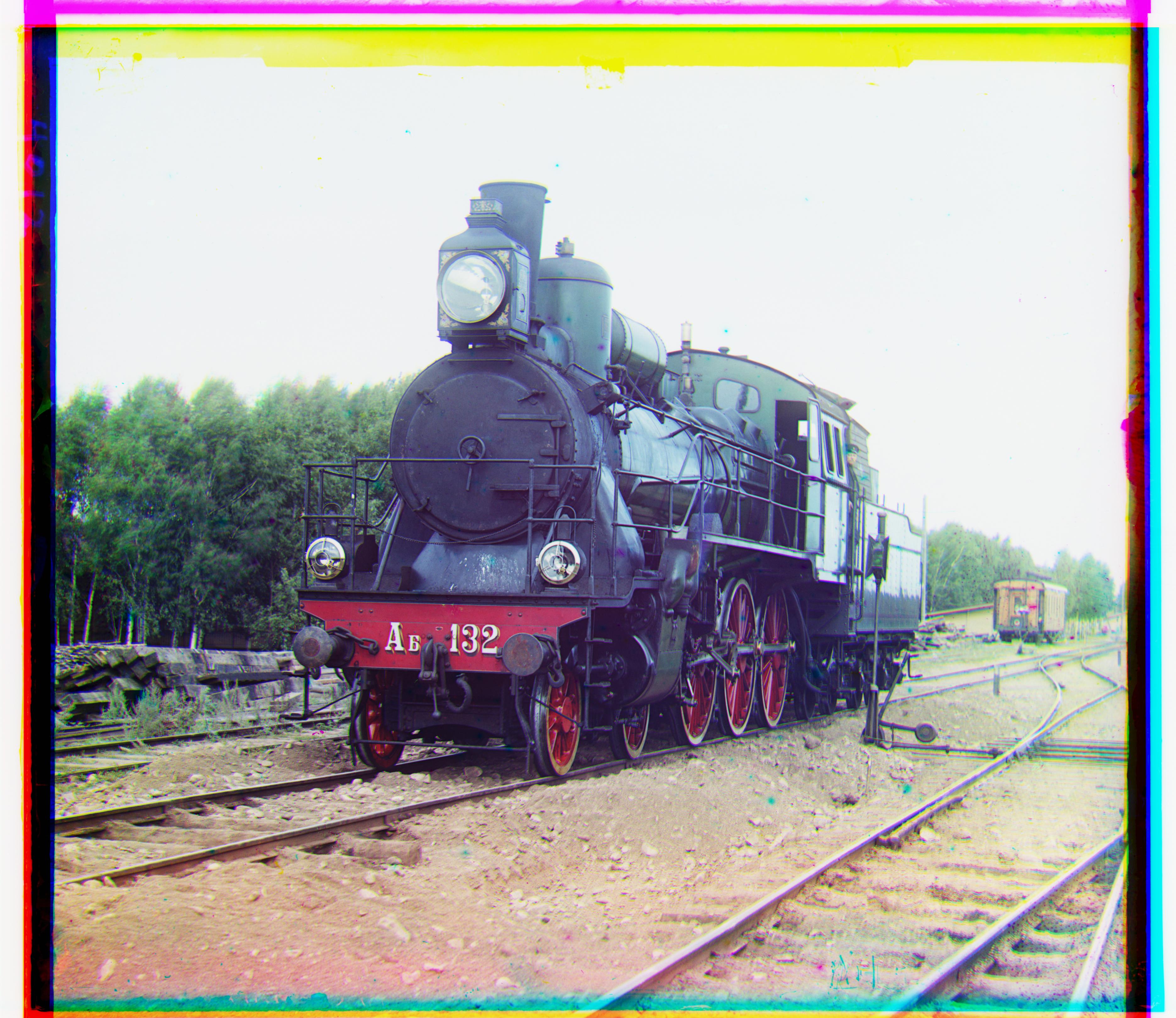
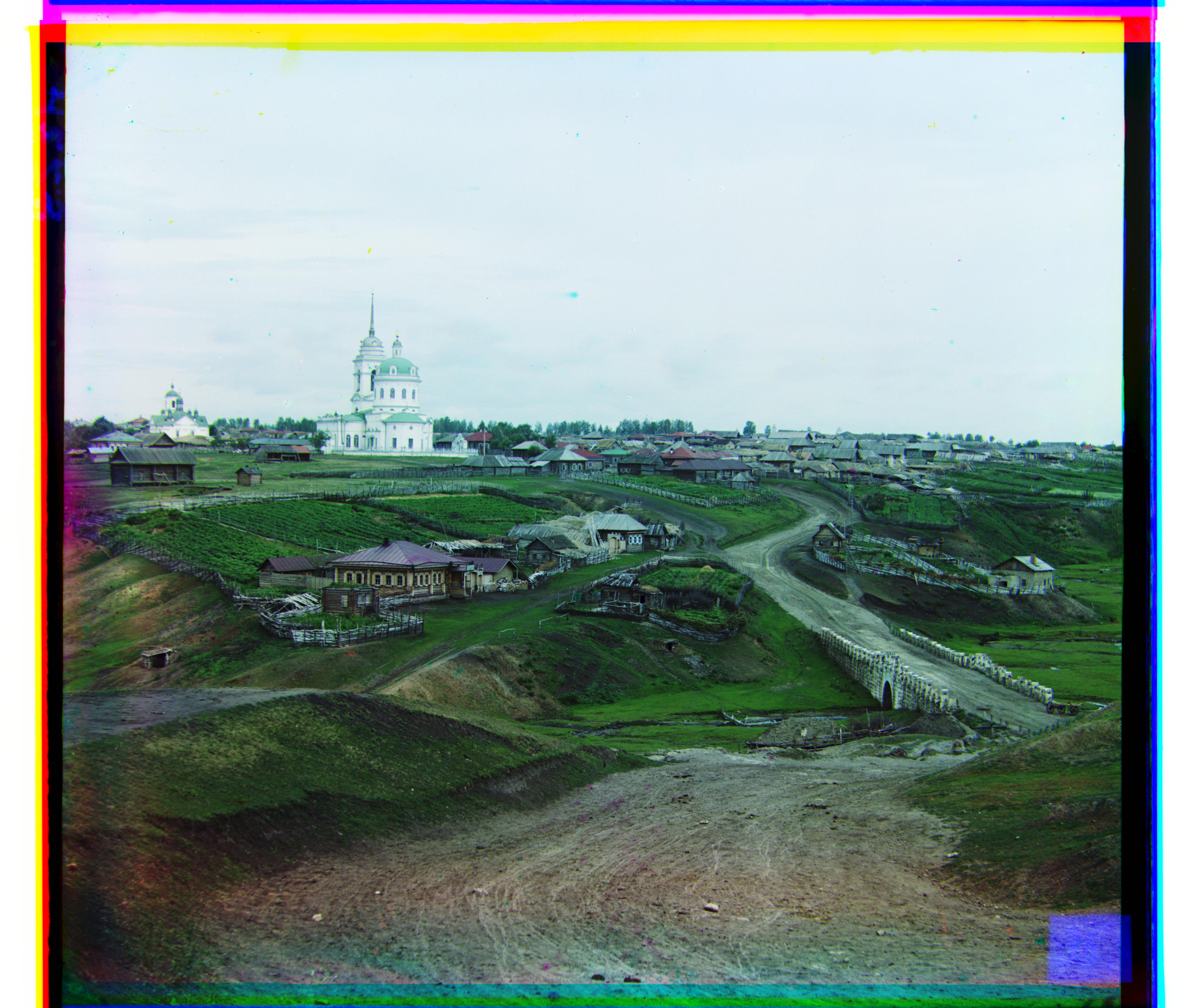
To align the images, we align images by maximizing a similarity metric across the three channels. We determine the optimum offset for the green and blue channels and then for the red and blue channels.
For each channel pair (green and blue, red and blue), we start with an exhaustive search of all combinations of vertical and horizontal offsets between -20 (left or up) and 20 (down or right). At each step, we compute the normalized cross-correlation (NCC). At the end of the search, we select the offset corresponding to the largest NCC score.
| Before | After | Green Offset (vertical,horizontal) | Red Offset (vertical,horizontal) |
|---|---|---|---|
|
|
(5,2) | (12,3) |
|
|
(-3,2) | (3,2) |
|
|
(3,1) | (7,0) |
|
|
(7,0) | (14,-1) |
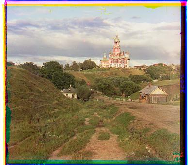
This approach works fine for smaller images, but for full size images (3683 × 9656), the vertical and horizontal search range of (-20, 20) is not enough. We need a search range of about (-200, 200), but this would mean that we need to search 401*401 = 160801 different offsets for each channel pair! To address this, we use an image pyramid algorithm.
We start by repeatedly scaling the image by a factor of 1/2 until we get to a size of (401 x 463), where a search range of (-20, 20) is sufficient. As before, we search all combinations of vertical and horizontal offsets between (-20, 20) and select the offset with the larged NCC score. We then scale up the image by 2 and then search the range of vertical offsets (prev_vertical_offset-1,prev_vertical_offset+1) and horizontal offsets (prev_horizontal_offset-1,prev_horizontal_offset+1). Repeat the until we scale the image back up to its original size.
| Before | After | Green Offset (vertical,horizontal) | Red Offset (vertical,horizontal) |
|---|---|---|---|
 |
 |
(49,24) | (103,44) |
 |
 |
(59,16) | (124,13) |
| (40,17) | (89,23) | ||
 |
 |
(47,9) | (112,11) |
 |
 |
(78,28) | (174,36) |
 |
 |
(53,14) | (111,11) |
 |
 |
(42,5) | (87,31) |
 |
 |
(56,21) | (116,28) |
 |
 |
(65,12) | (137,22) |
 |
 |
(71,17) | (152,24) |
 |
 |
(69,31) | (136,49) |
 |
 |
(27,-26) | (106,-51) |
 |
 |
(17,12) | (31,14) |
 |
 |
(68,24) | (144,38) |
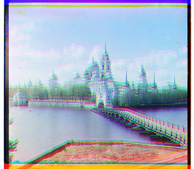
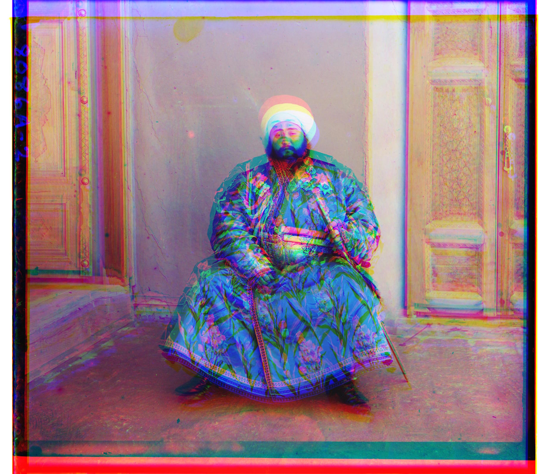
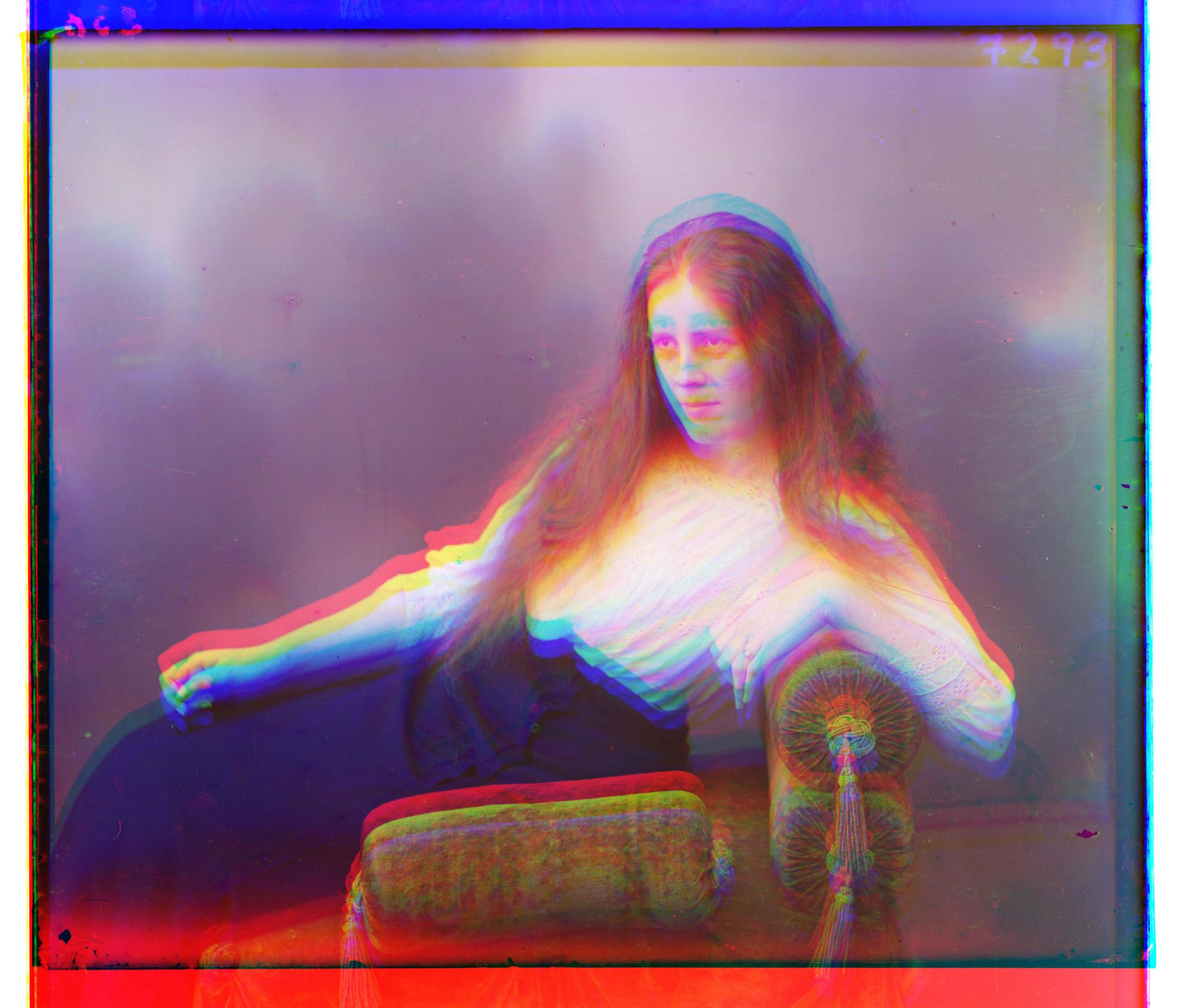
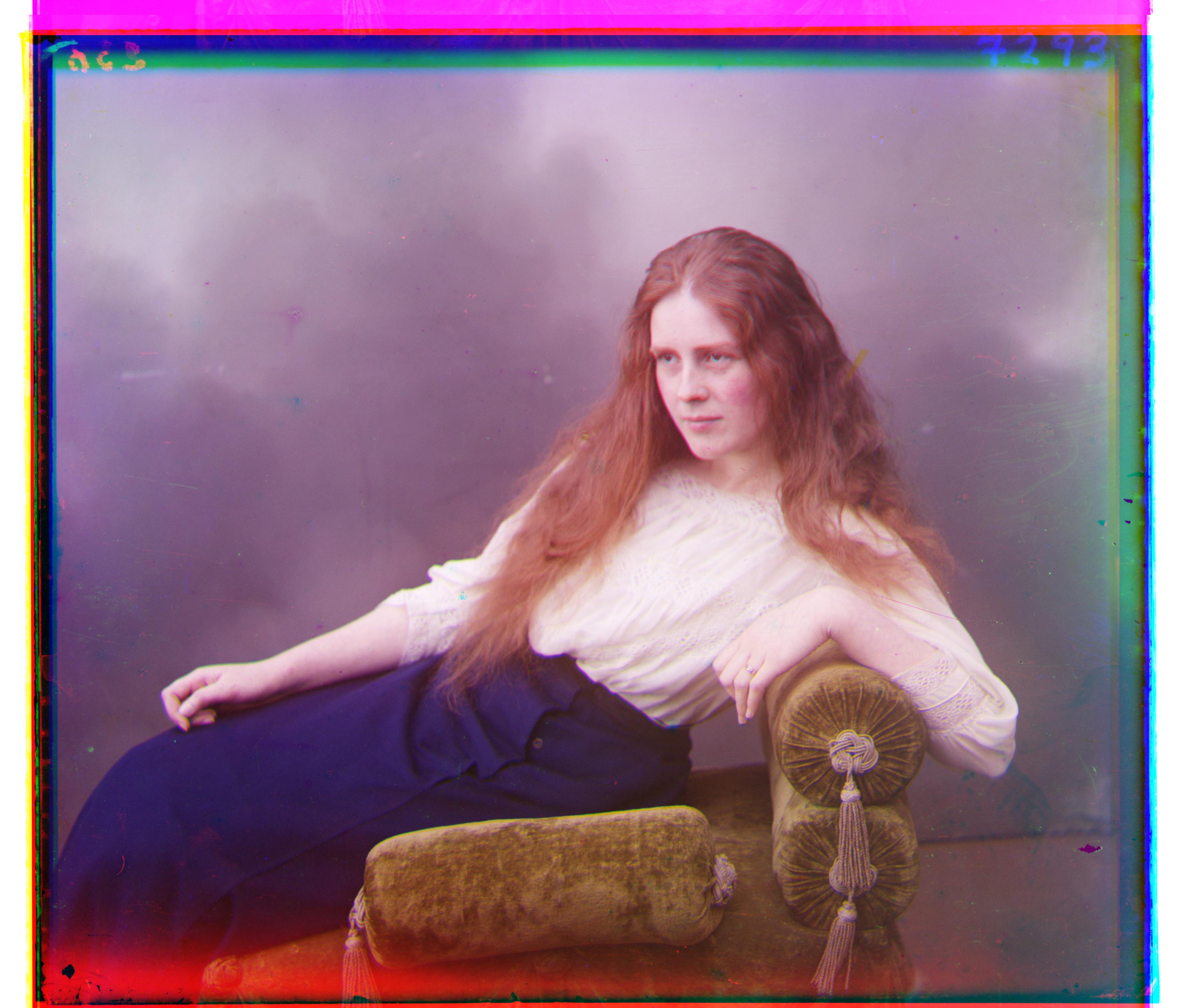
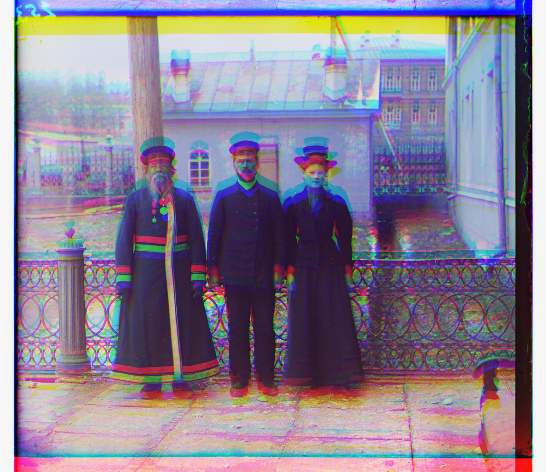
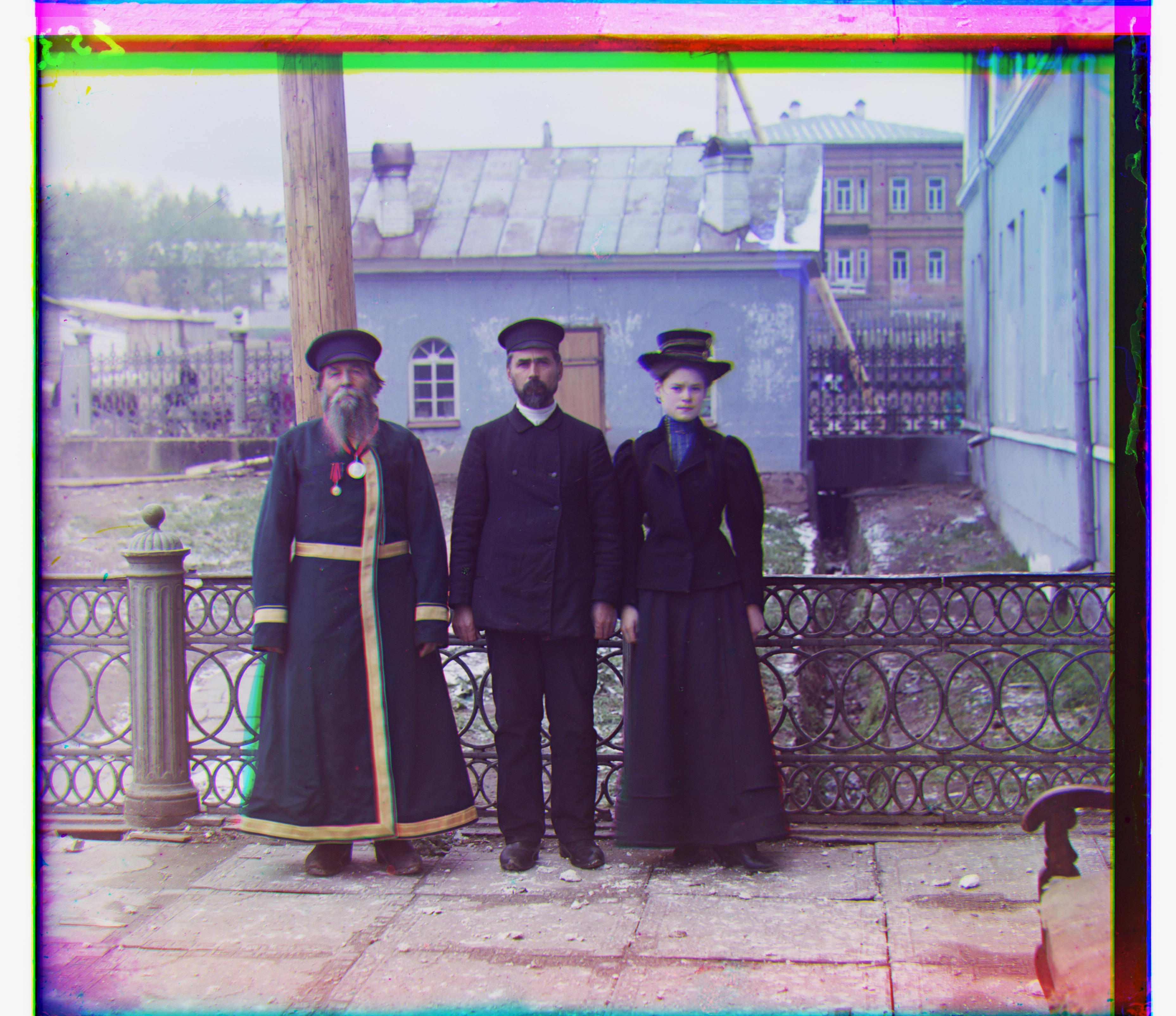
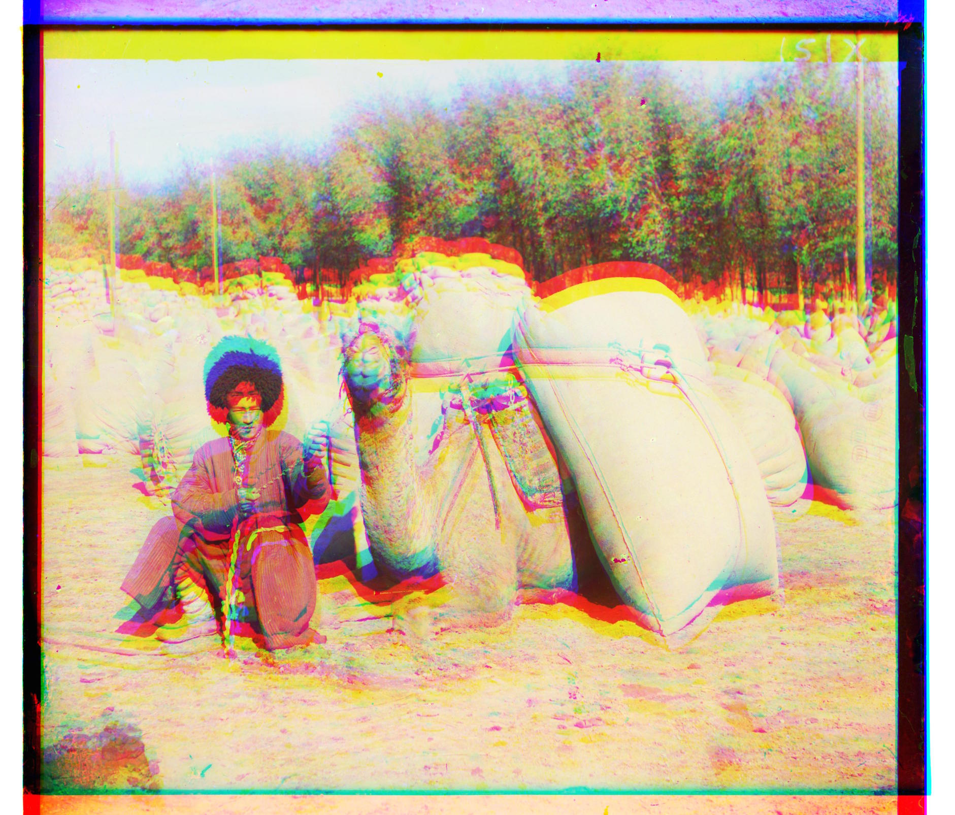
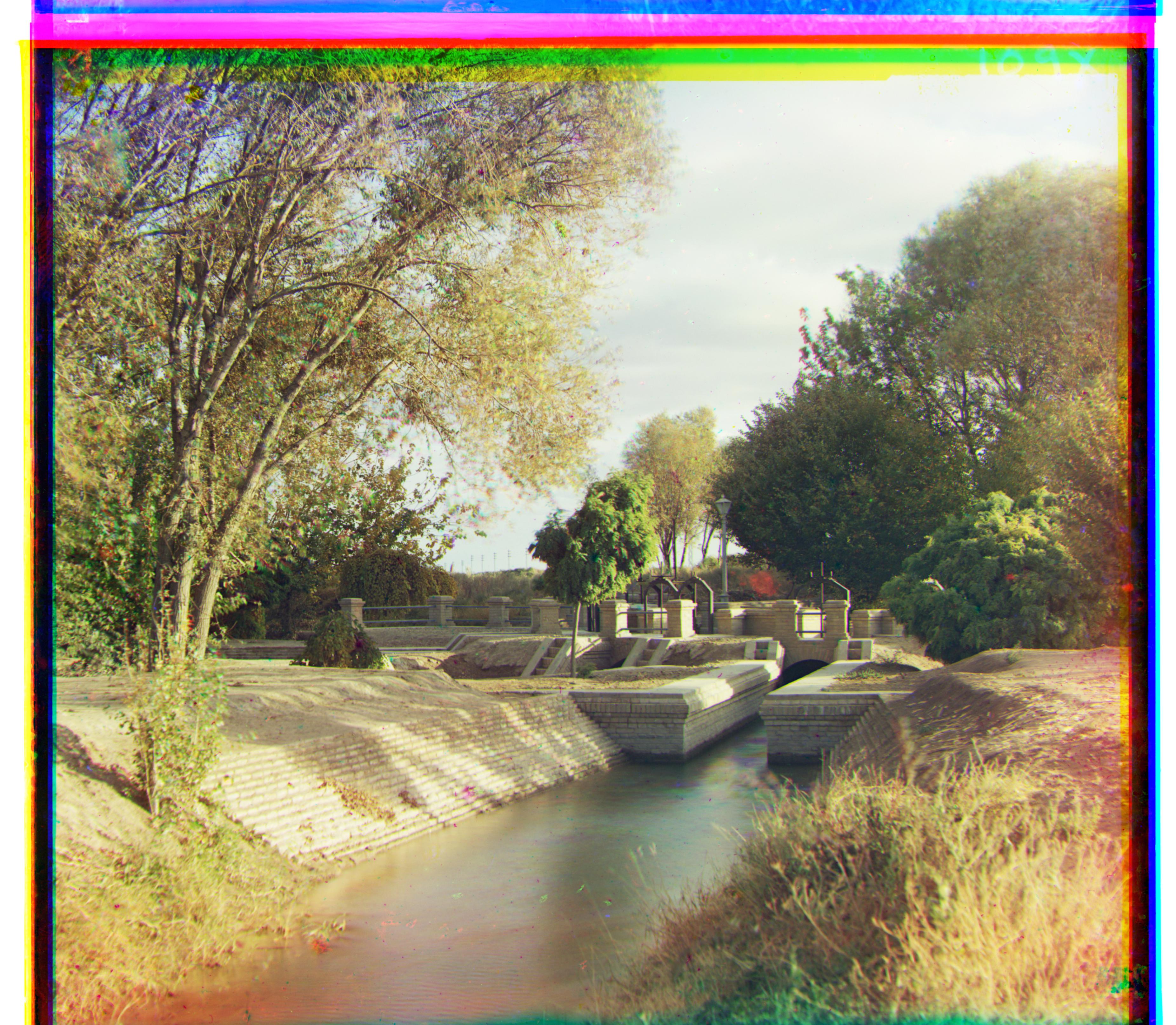
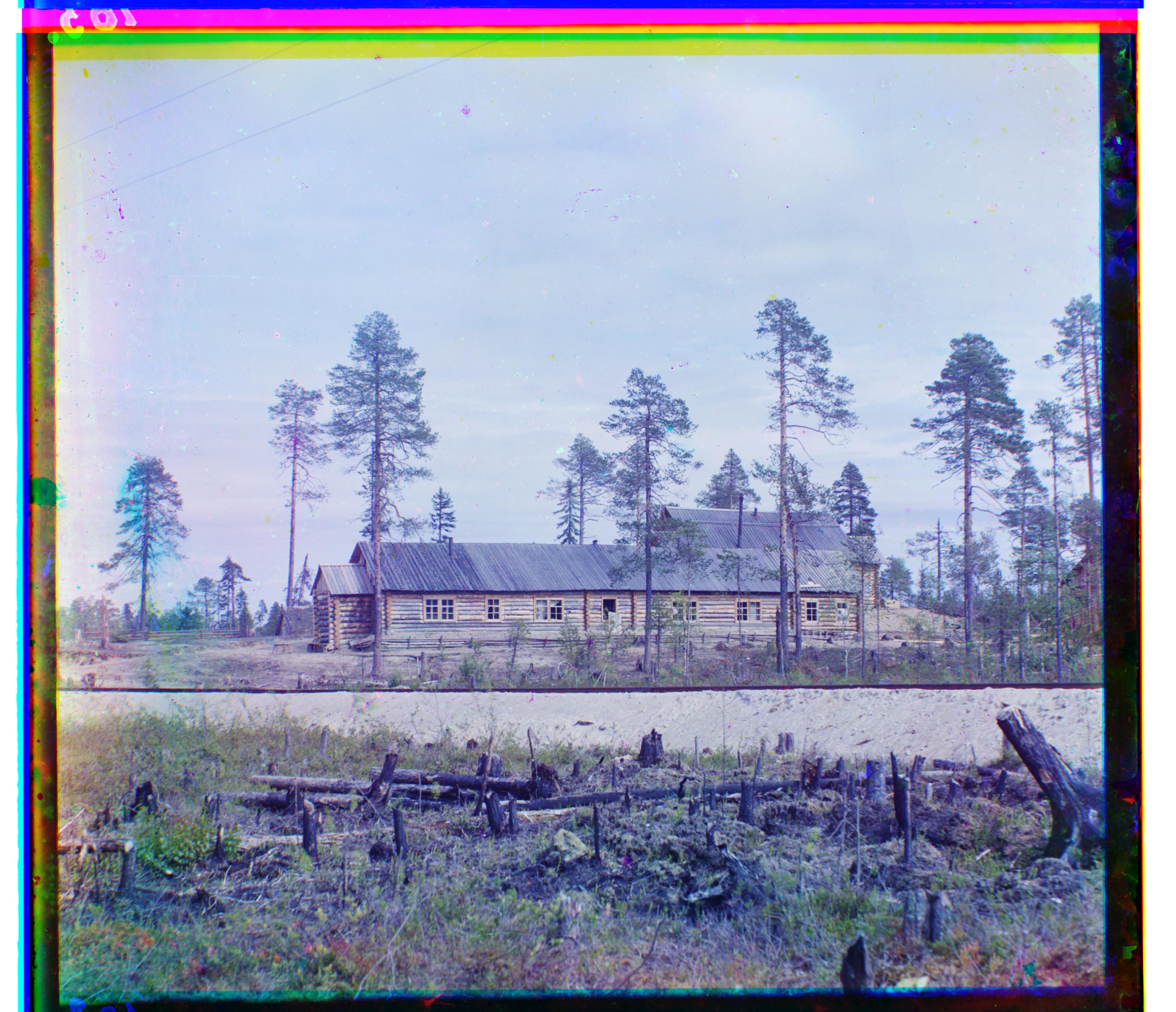
You'll notice that all of the images above have both black and colored borders-- even the aligned ones. The black borders are from imperfect cropping of the source scans. The colored borders are the result of one or more of the color channels being damaged at the edges (after all, these glass plate negatives are more than a hundred years old). In order to trim off these odd-colored borders, we used a two-stage cropping process.
First, we trim off the edges of the image where one or more of the channels has no data. For example, if the green channel needed to be offset from the blue 10 pixels down and 20 pixels right, then we would trim off 10 pixels from the top and bottom of the image and 20 pixels from the left and right of the image. We also consider the red channel vs. the blue and trim according to the max vertical and horizontal offsets of the green vs. blue and red vs. blue.
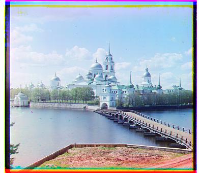
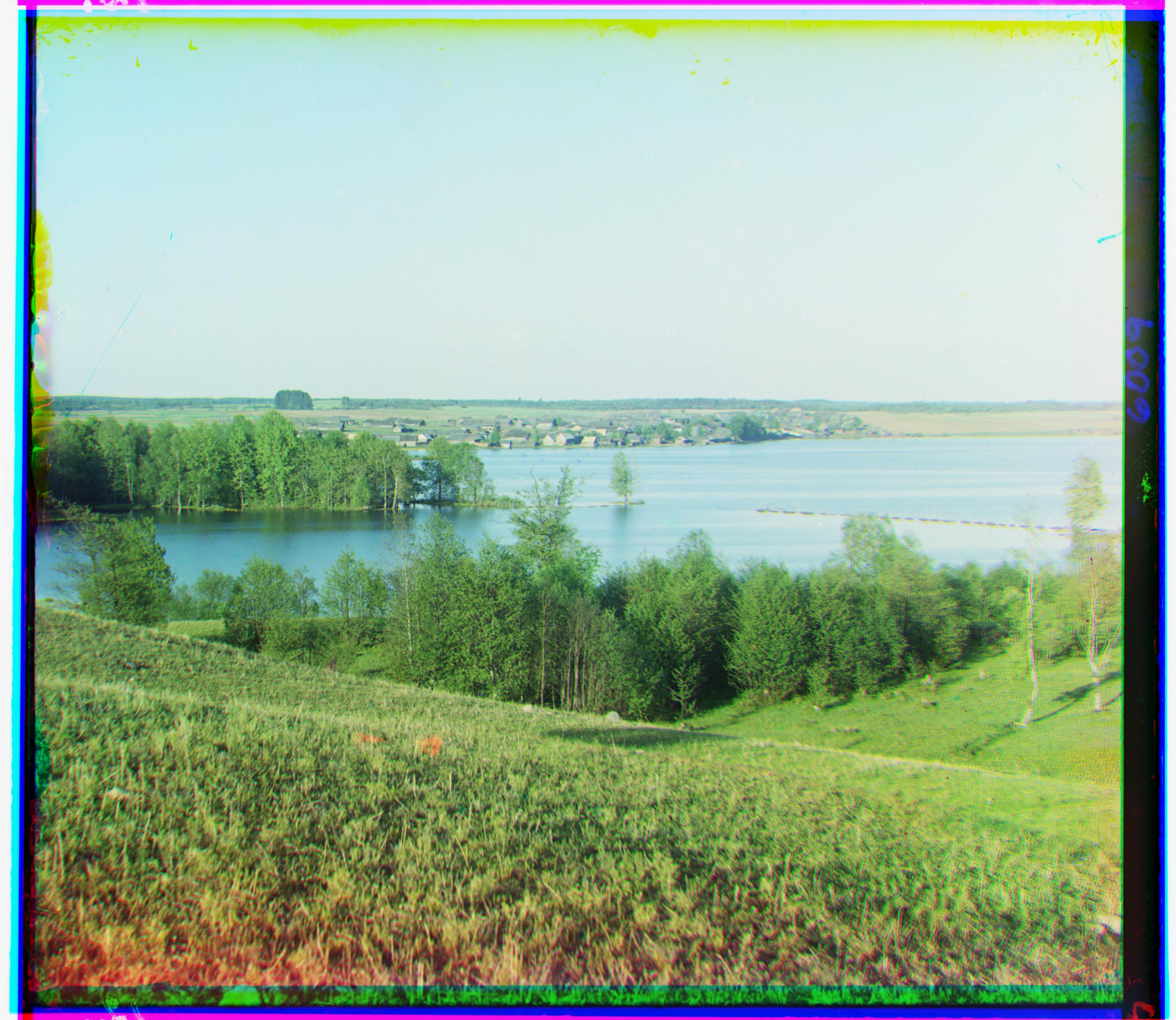
The first step described above works okay, but a lot of the borders remain because it does not get rid of the borders caused by imperfect cropping of the source scans. For the next stage of cropping we use a very naive technique for edge detection. We process the top, bottom, left, and right 1/8 (this is a parameter that can be adjusted; 1/8 was chosen because it is unlikely that a border will extend more than 1/8 of the height or width of an image). If we're processing the right side of the image for example, we take the average of each column of pixels. This effectively squishes (vertically) the right 1/8 block of the image into a single line of pixels. Now that we're working with a one-dimensional list, we iterate from left to right, and we record the index where we first see a pixel intensity value drop more than 1/2 from its neighbor. This large dropoff indicates that we've likely encountered a border, where pixel intensity values are closer to 0 than 1. We use the index determined from this algorithm (repeated for all sides and all color channels) to slice off the offending edges of the images. As you can see below, it works pretty well:
| Before Crop | After Crop |
|---|---|
|
 |
|
 |
|
 |
|
 |