Getting Started
The package is written in Python 3 and requires a recent version of numpy and scikit-image. Invoke the main.py file to run each tool.
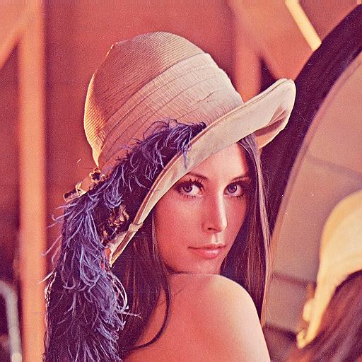
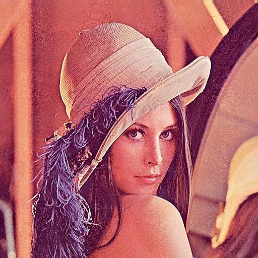
Unsharpening
We implement the well-studied unsharp masking image sharpening technique. A blurred, or "unsharp", copy of the image is used to extract high frequency components which is then added back to the original image to enhance the perceptual sharpness.

Hybrid Images
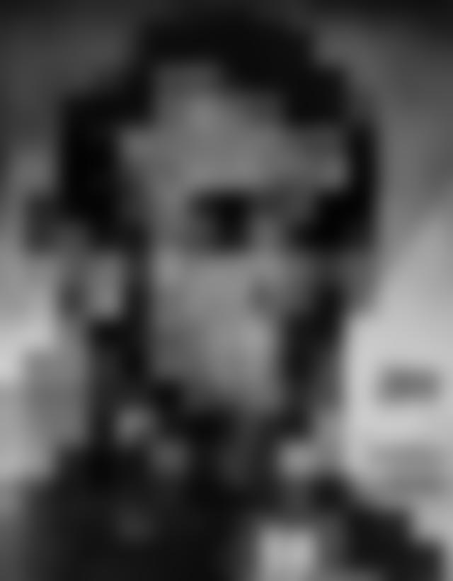
Hybrid images are static images that change in interpretation as a function of the viewing distance.
Human perception is sensitive to different frequencies at different distances. High frequency components tend to dominate visual perception when visible, but as the viewer draws away and the high frequency details are no longer perceived, the underlying low frequencies are revealed.
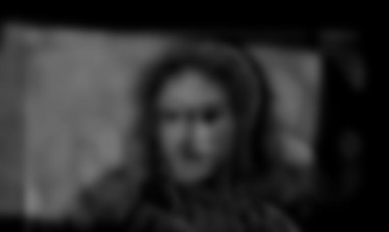
A well-known example is Salvador Dali's Gala Contemplating the Mediterranean Sea which at Twenty Meters Becomes the Portrait of Abraham Lincoln.
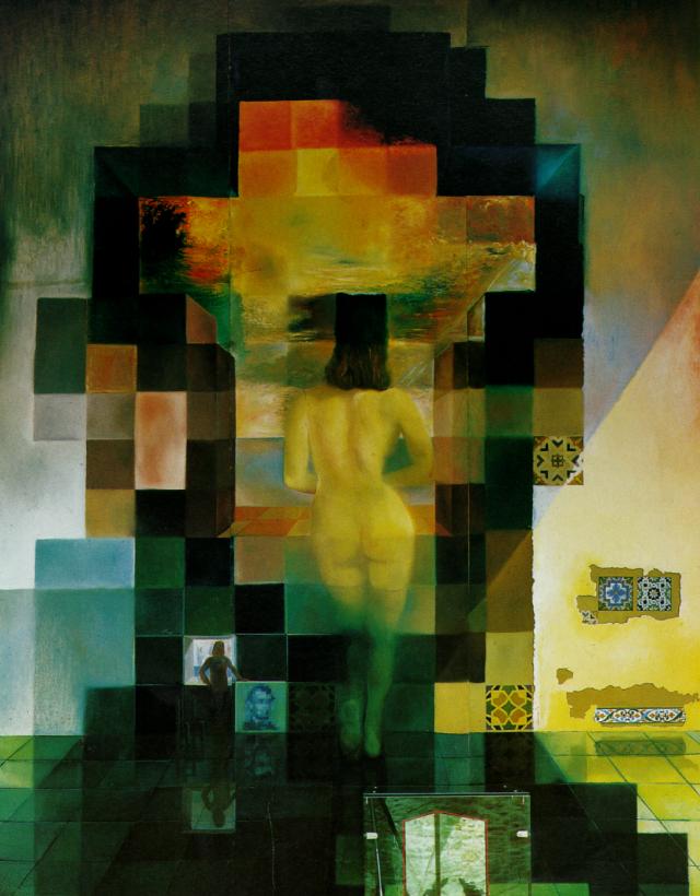
We emulate Dali's frequency domain effects by combining the high frequency components of one image with the low frequency components of another. To improve the effect, it is necessary to align the images to reduce visual discontinuities. This was done by collecting user input.
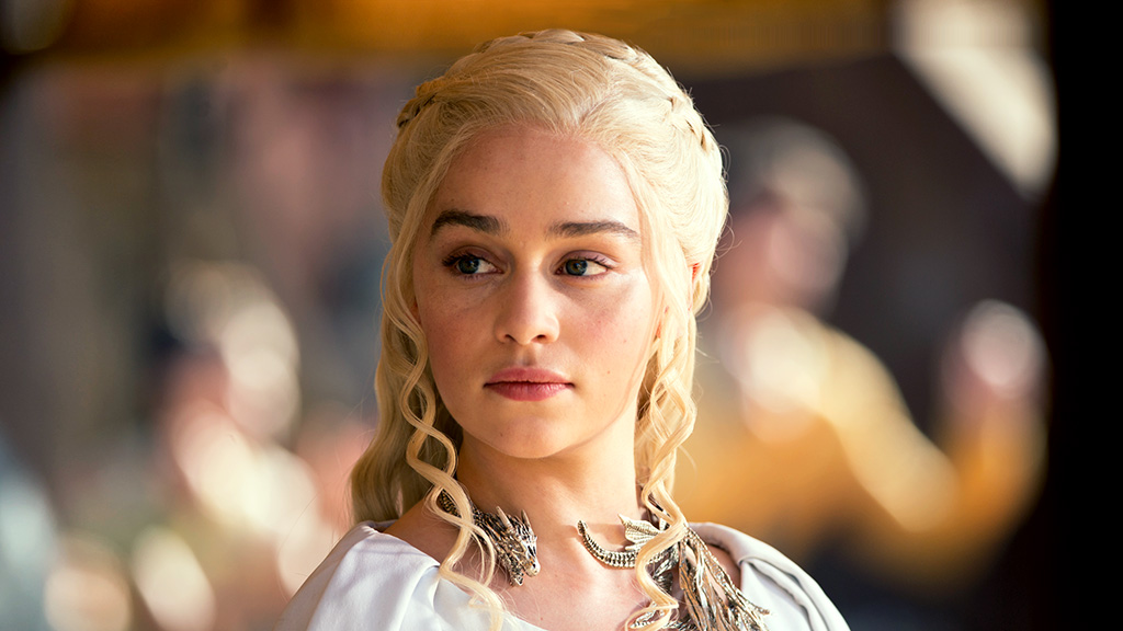
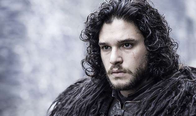
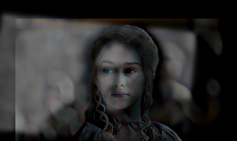

The filtered image analysis provides better insight into which components of the final image are from Jon and which components are from Daenerys.
From the examples we tried, we believe that color enhances the effect for the high frequency components, but tends to distract and contribute less for low frequency components.
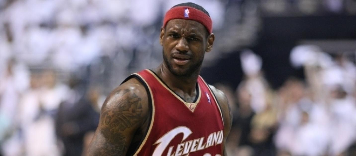
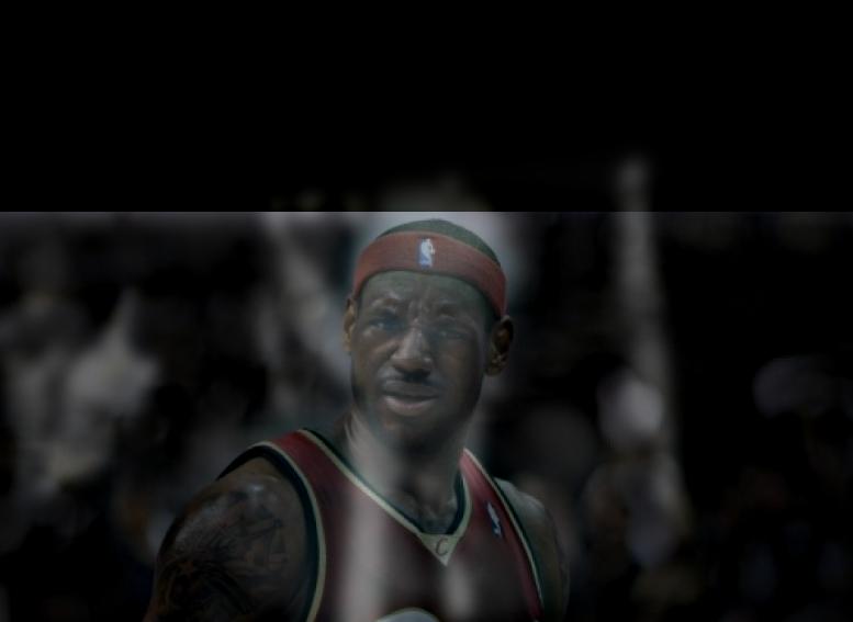
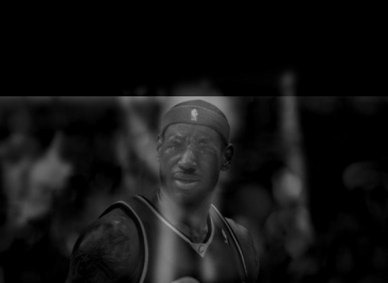
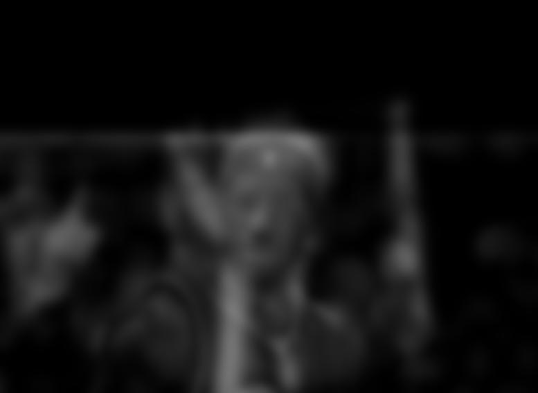
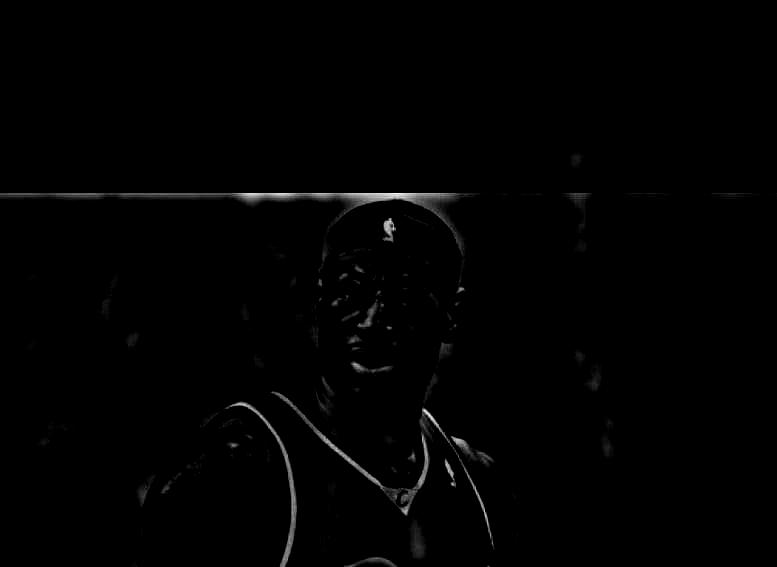
We also created another image featuring LeBron and Trump, but LeBron's disappointment and facial features seem to overshadow Trump's anger in the low frequencies even when viewing the hybrid image from afar.

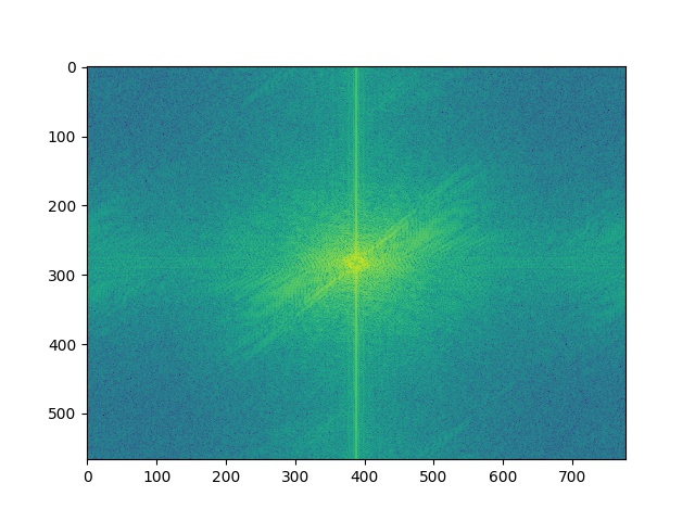
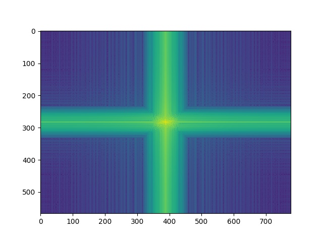
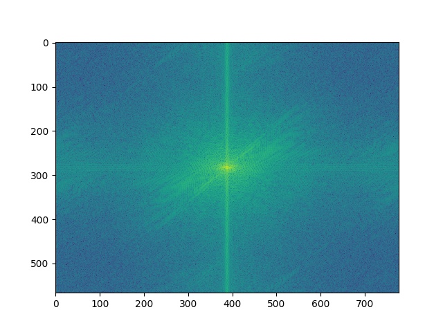
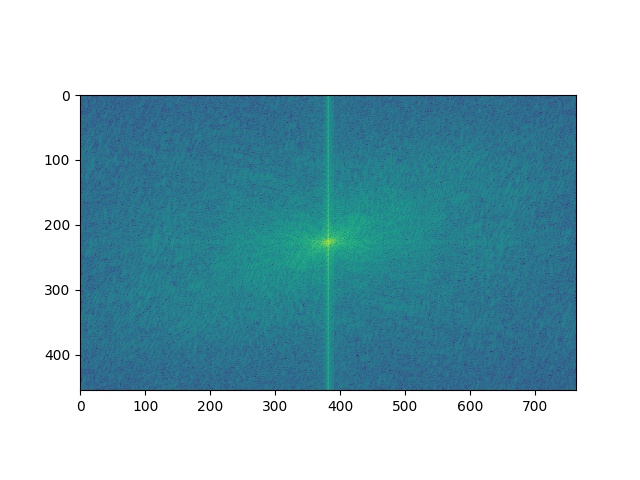
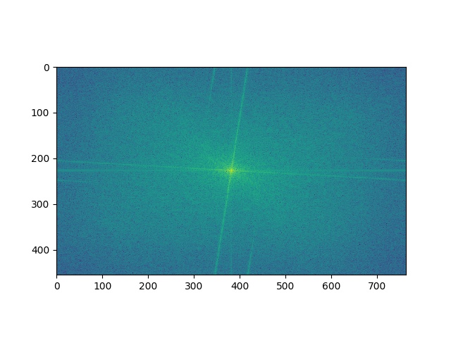
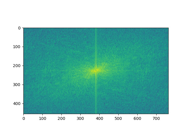
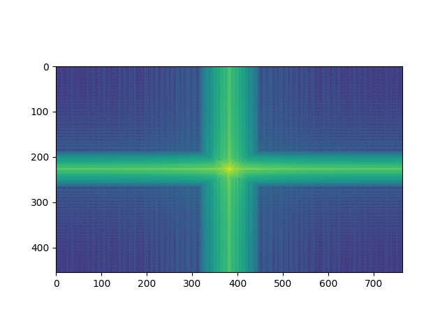
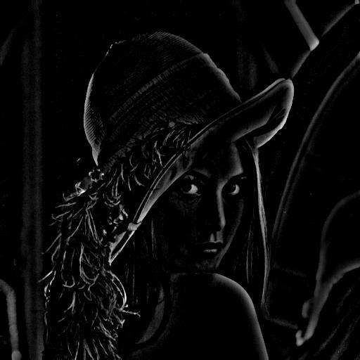
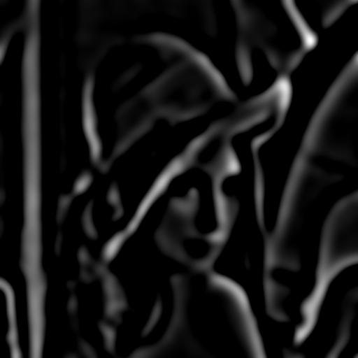
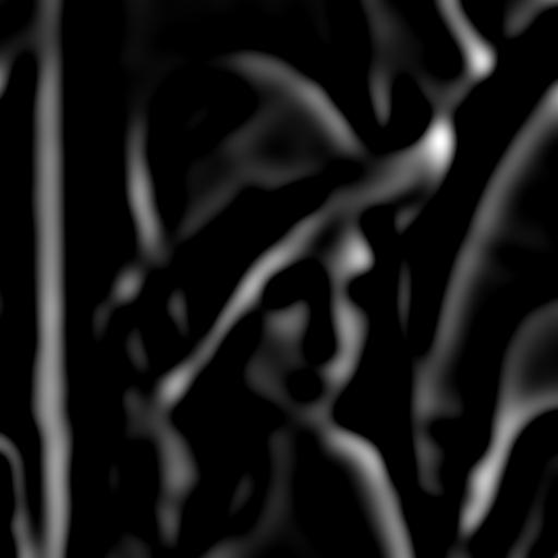
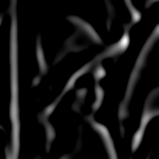
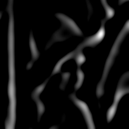
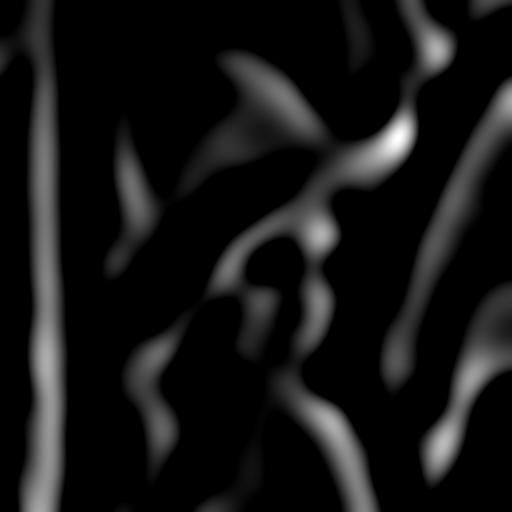
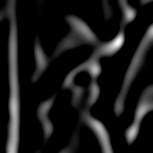
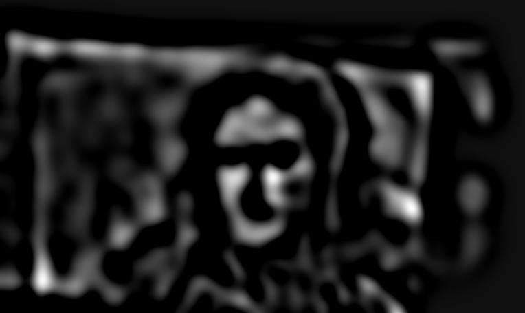
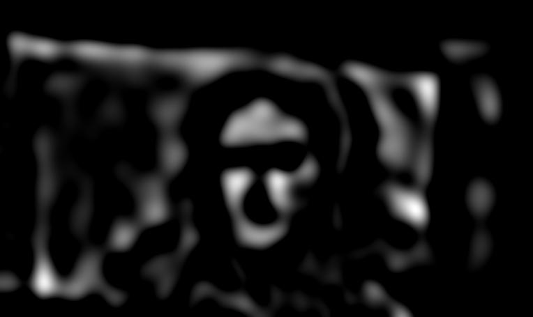
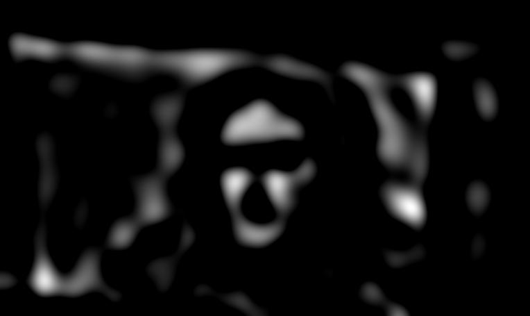
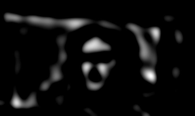
Frequency Stacks
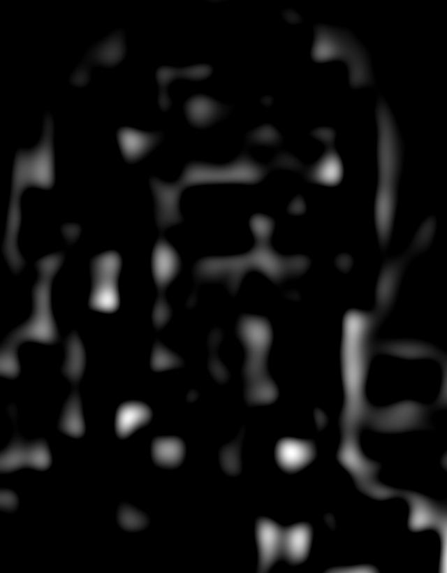
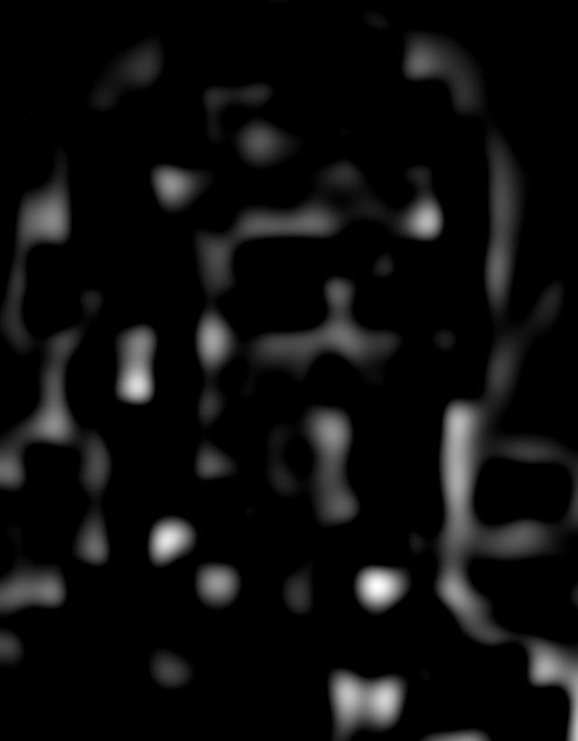
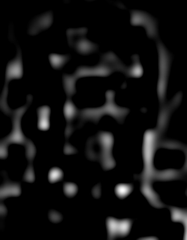
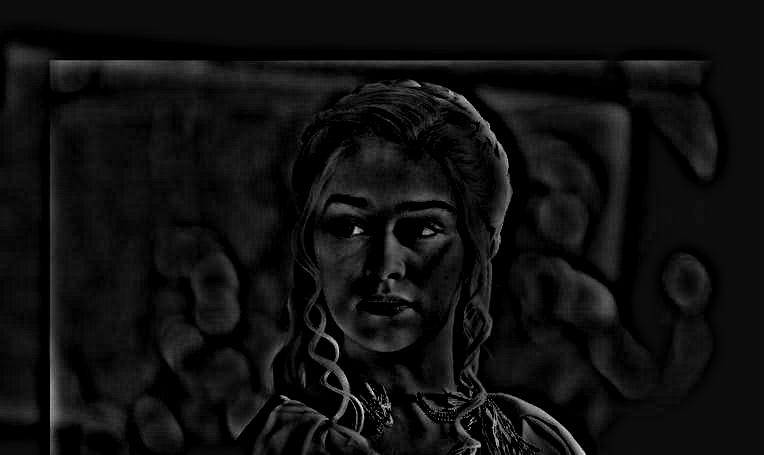
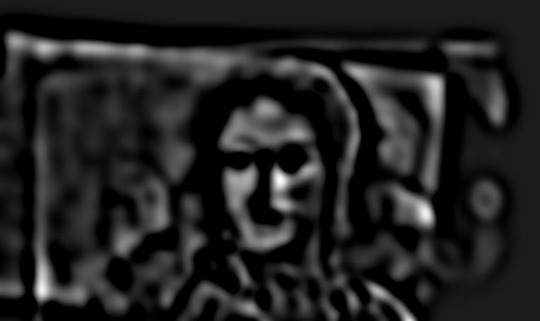
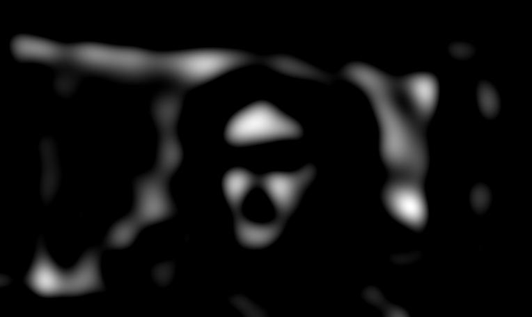
To help analyze and interpret the visual results of frequency domain blending, we visualized each image's Gaussian and Laplacian stacks. Gaussian stacks are the result of repeatedly applying a gaussian filter over the source image, yielding blurrier and blurrier images. The Laplacian stack builds from the Gaussian stack by finding the difference between adjacent blurred images in the stack. This difference represents the amount of information captured by a particular frequency band.
To line up results, we repeat the final Gaussian layer in the Laplacian stack results.


Multiresolution Blending
An image spline is a smooth seam joining two image together by gently distorting them.
Multiresolution blending computes a gentle seam between the two images seperately at each band of image frequencies, resulting in a much smoother seam.
A Toy Problem
[T]he gradient is a multi-variable generalization of the derivative. While a derivative can be defined on functions of a single variable, for functions of several variables, the gradient takes its place...
In the case of images, gradients work like 2D derivatives. Gradient domain processing starts from a simple principle: instead of recording individual pixel intensities, we can instead record neighboring gradients to capture the same information. In fact, we can fully express an image using only the gradients a single intensity to recover the constant factor lost during derivation.
These results were obtained from formulating a system of linear equations, each equation representing a single pixel's gradient x-direction or y-direction constraint. We then used a linear system solver to compute the original image subject to the additional constraint that the upper left corner of the image matches the input.

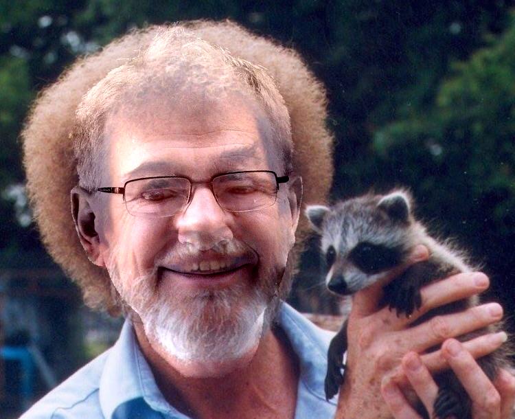
Poisson Blending
Poisson blending extends on our existing frequency domain blending techniques which left much to be desired. If our only constraint is the gradient, or details that change across an image, then Poisson blending may be the better technique.
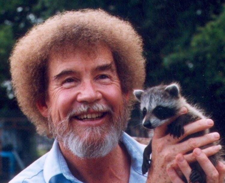
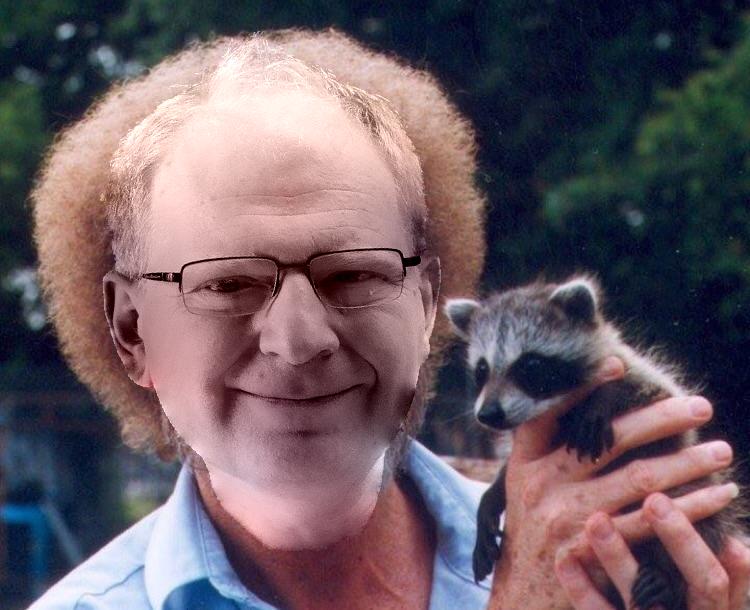
Let's start by comparing some of the results. On the left is our baseline image splining multiresolution blending technique. While it does a good job with preserving interior details, there is a harsh discontinuity between Bob Ross's face and Efros's face. The standard Poisson blend improves on texture matching, but still can't quite overcome the differences in color and intensity especially around the neck area.
Finally, we also developed a mixed blending method to allow adaptive transparency from the target image (the background). In the mixed blending mode, instead of universally preferring the masked source image gradients, we instead choose the stronger of the taret and source image gradients to help preserve existing details in the target image that might be overwritten by lower-intensity graphics in the source image.
None of the techniques, however, seem to work well with Efros and Ross due to the great disparity in lighting conditions and visual continuity. Even after manipulating the mask, we weren't able to significantly improve the result: the source images are too different.
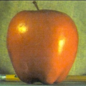
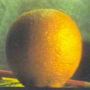
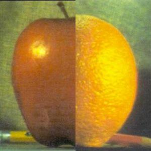
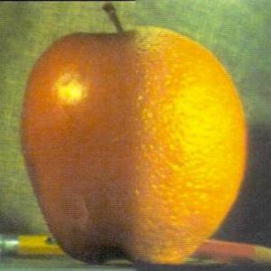
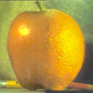
We also revisited the 'orapple' from earlier. Notice how the color of the apple is a little different: it's assimilated into the orange as part of the gradient.
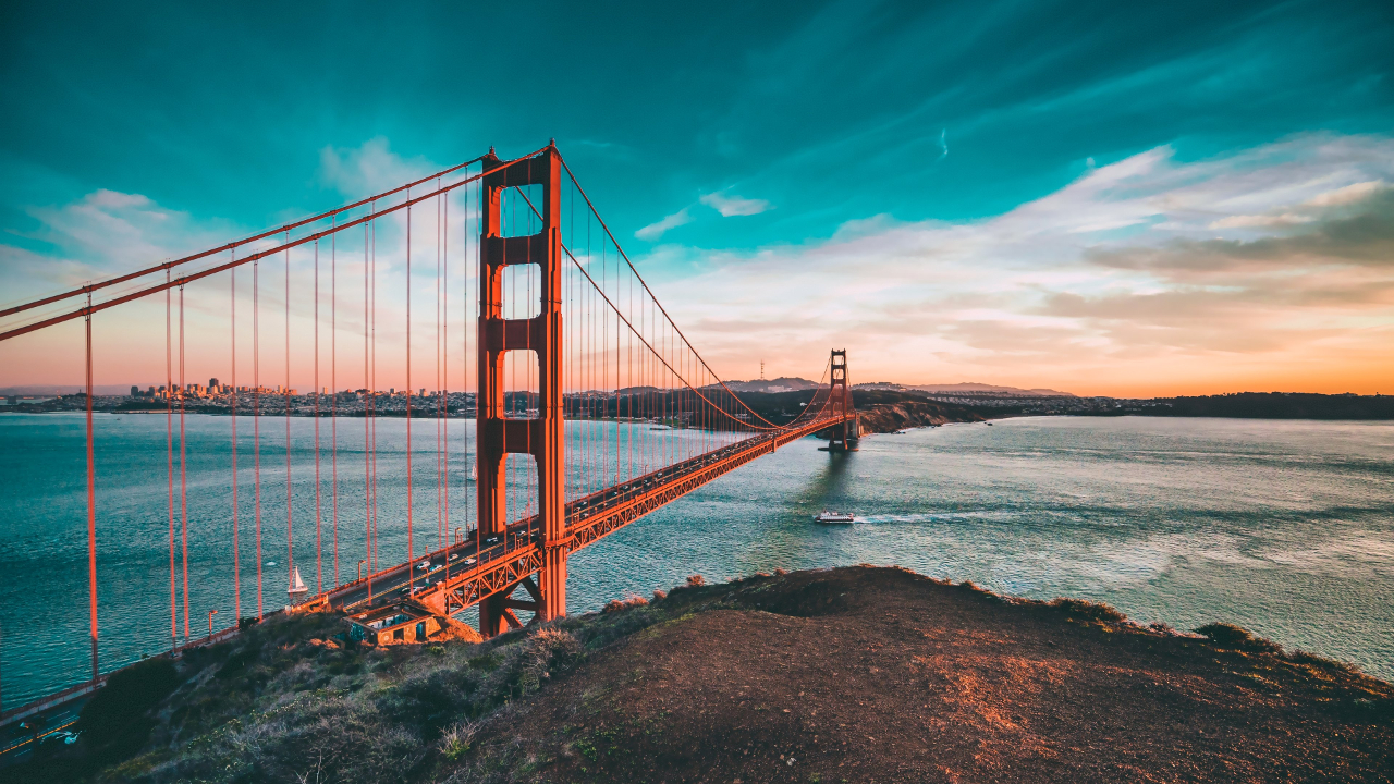
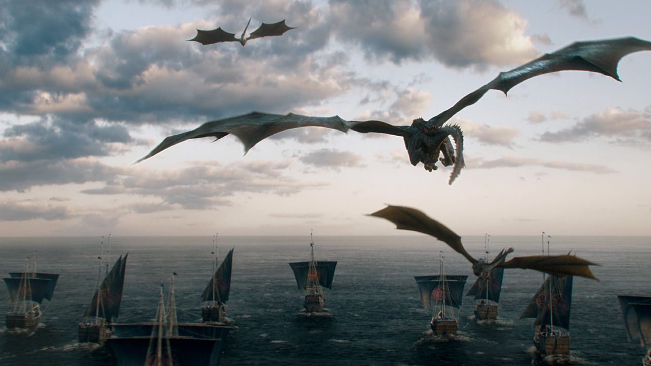
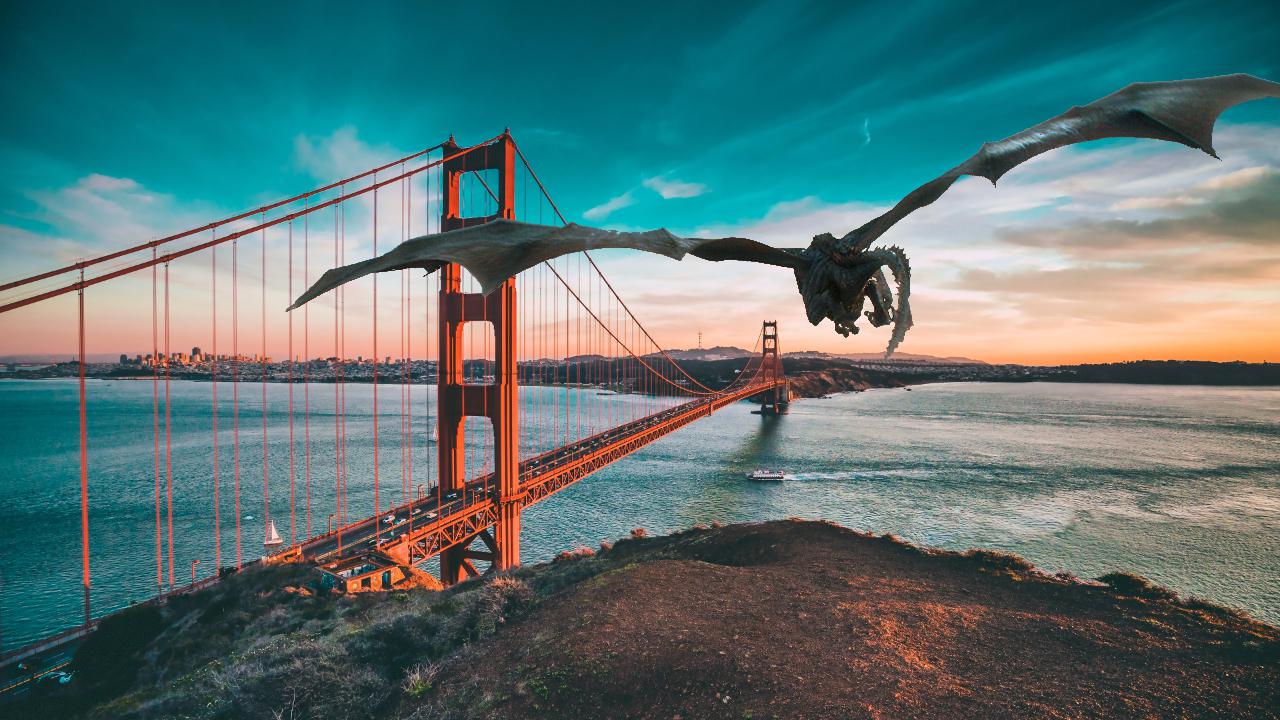
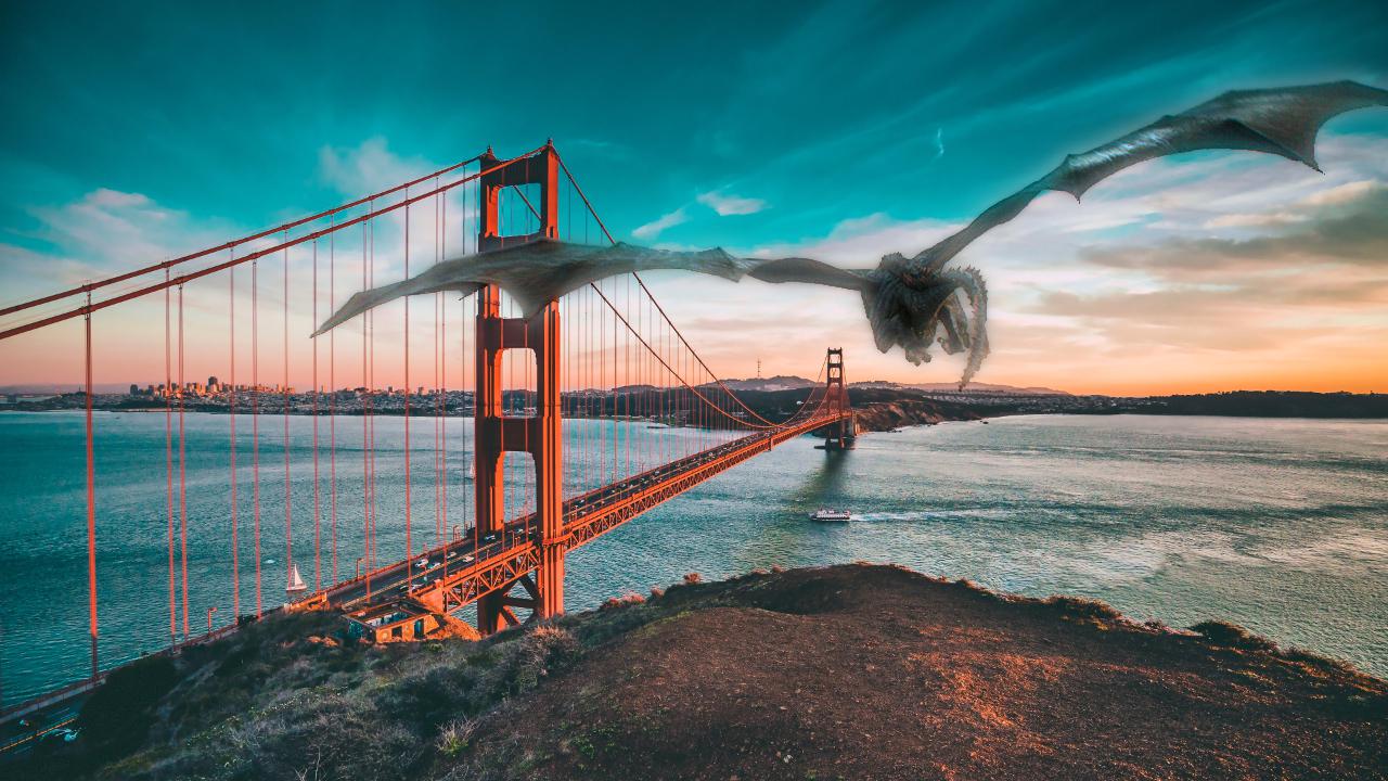
Our favorite blending result combined a sunset with the dragon from before.
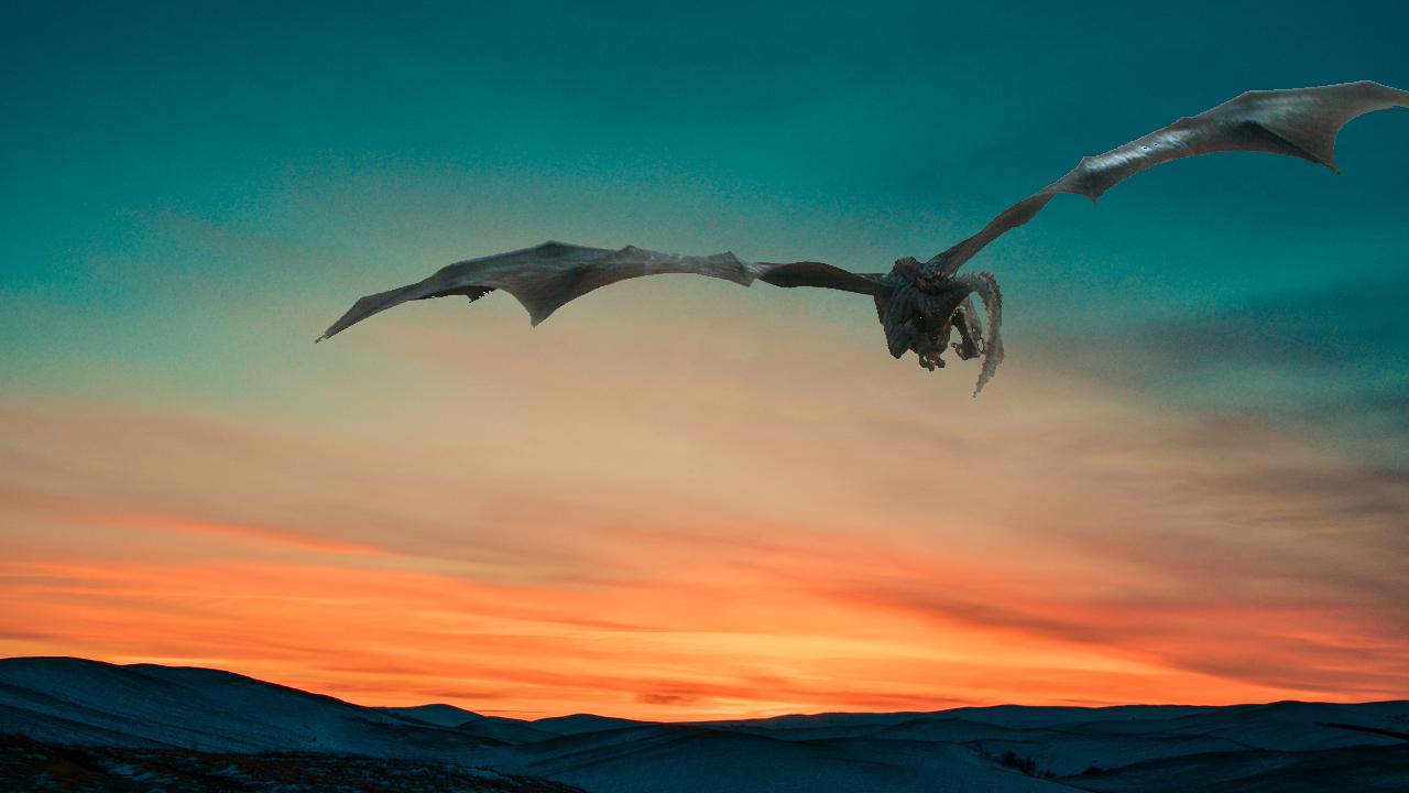
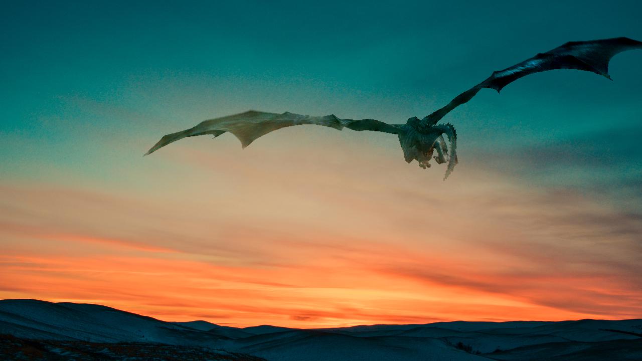
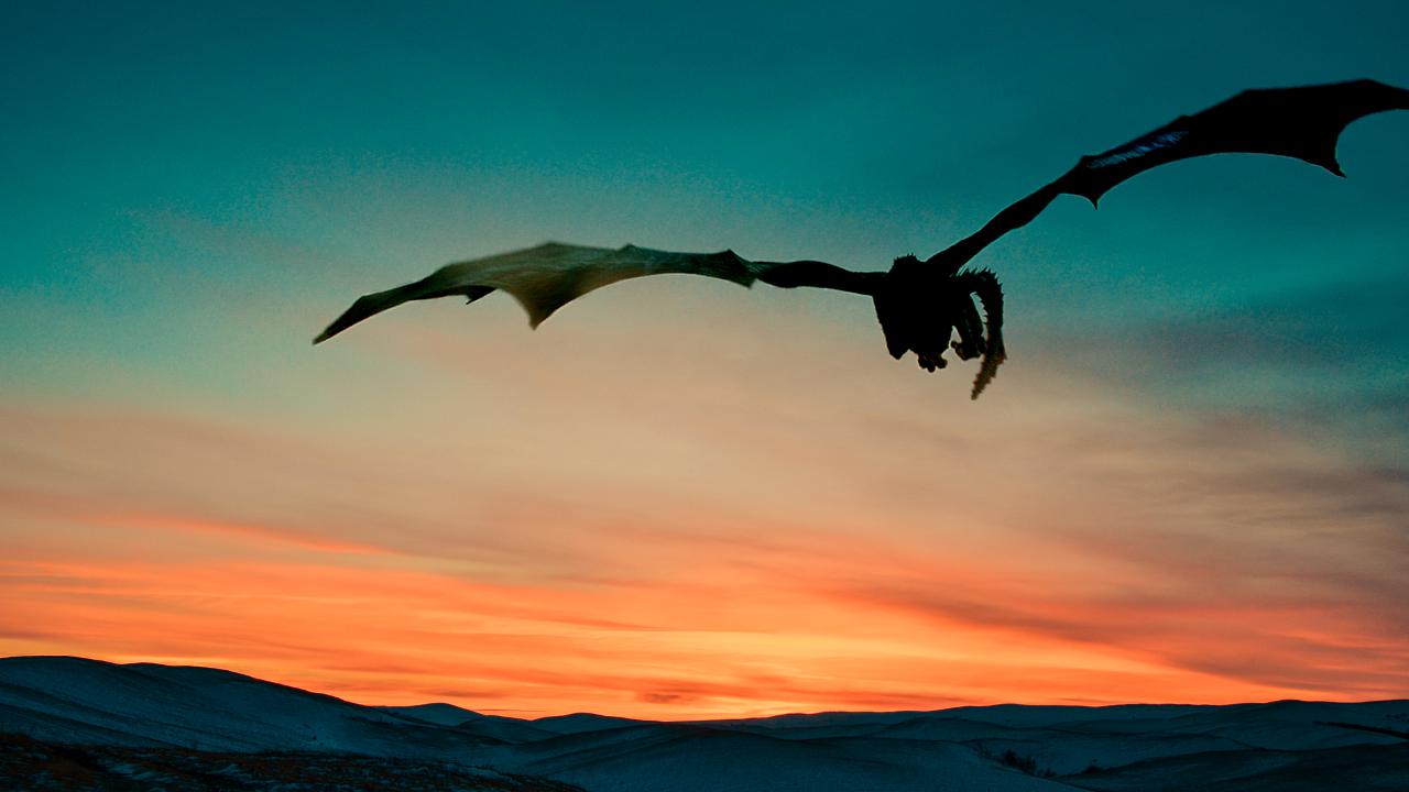

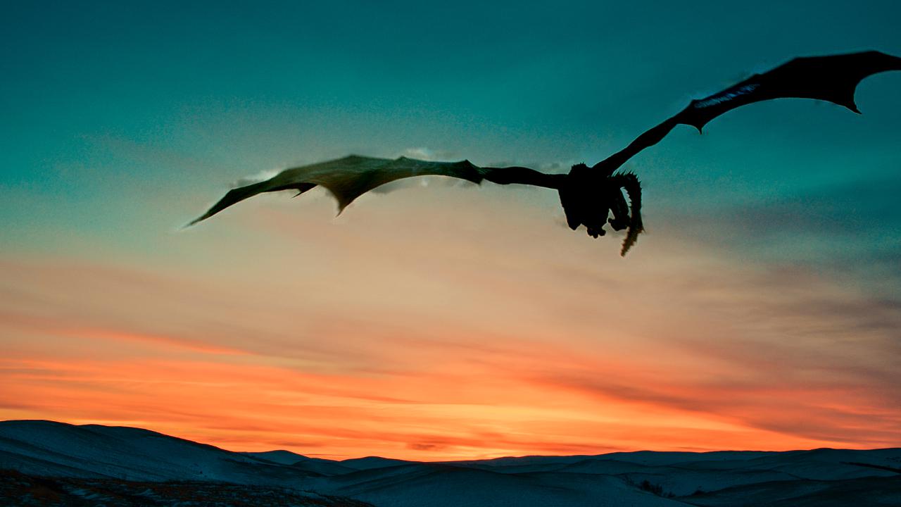

The close mask (as used in the multiresolution blend earlier) doesn't look right: the gradient solution is attempting to smooth over the colors and intensities of the sky so as to match the color of the dragon whereas the dragon should be an entirely different color.
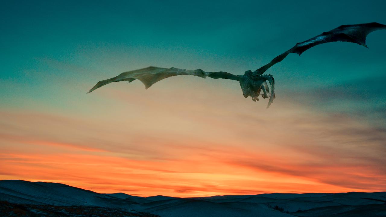
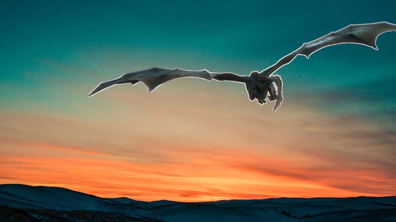
The 3px 'expanded' mask turned out the best. The dragon's original background sky isn't perceptible as it's hidden under the contour of the dragon, but it also serves as a buffer for the gradient solution to smoothly adjust for the lighting difference.
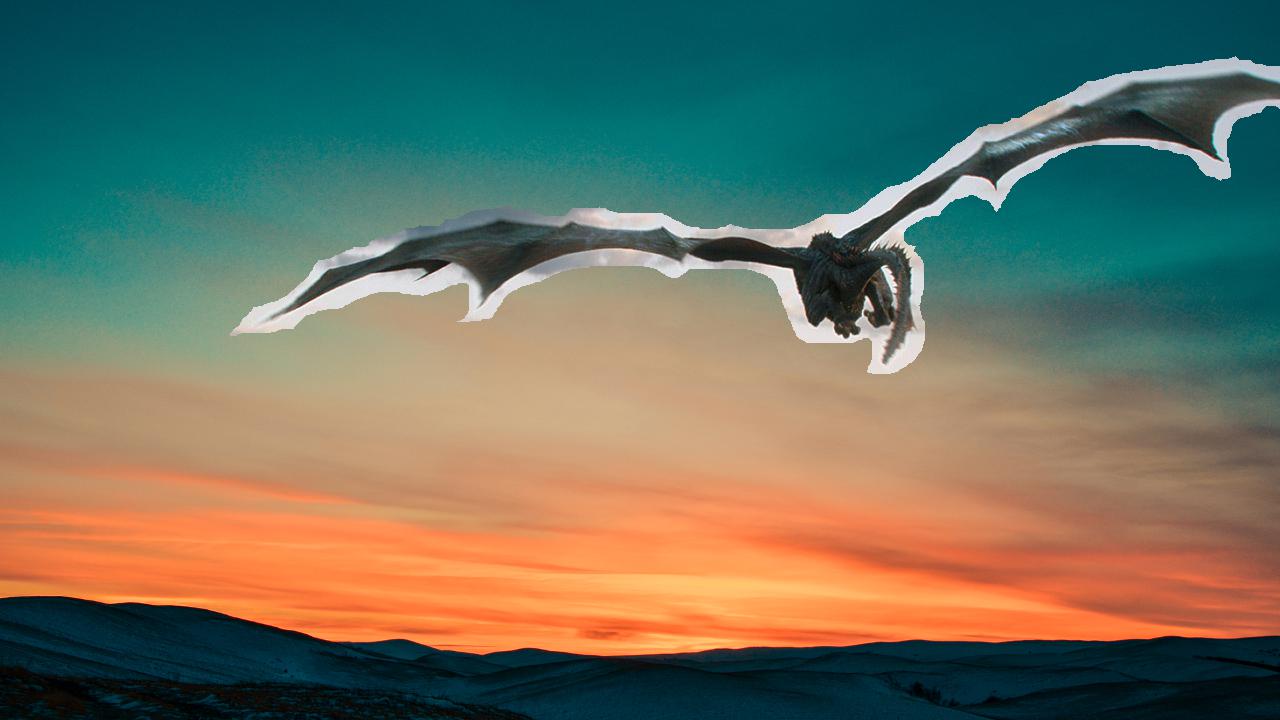
But in the case of the very wide mask, the original background begins to leak through. Mixed blending doesn't help in this situation as the sunset background is a fairly low gradient.
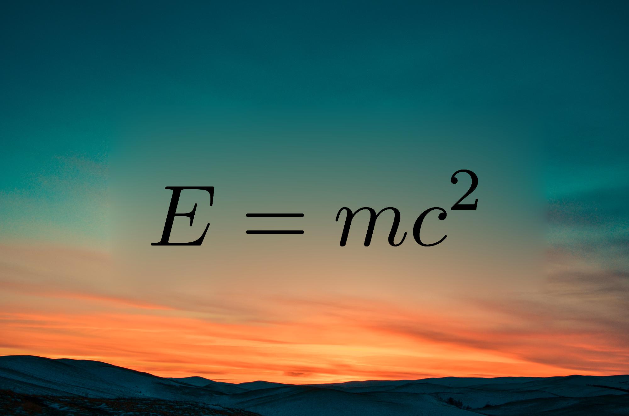
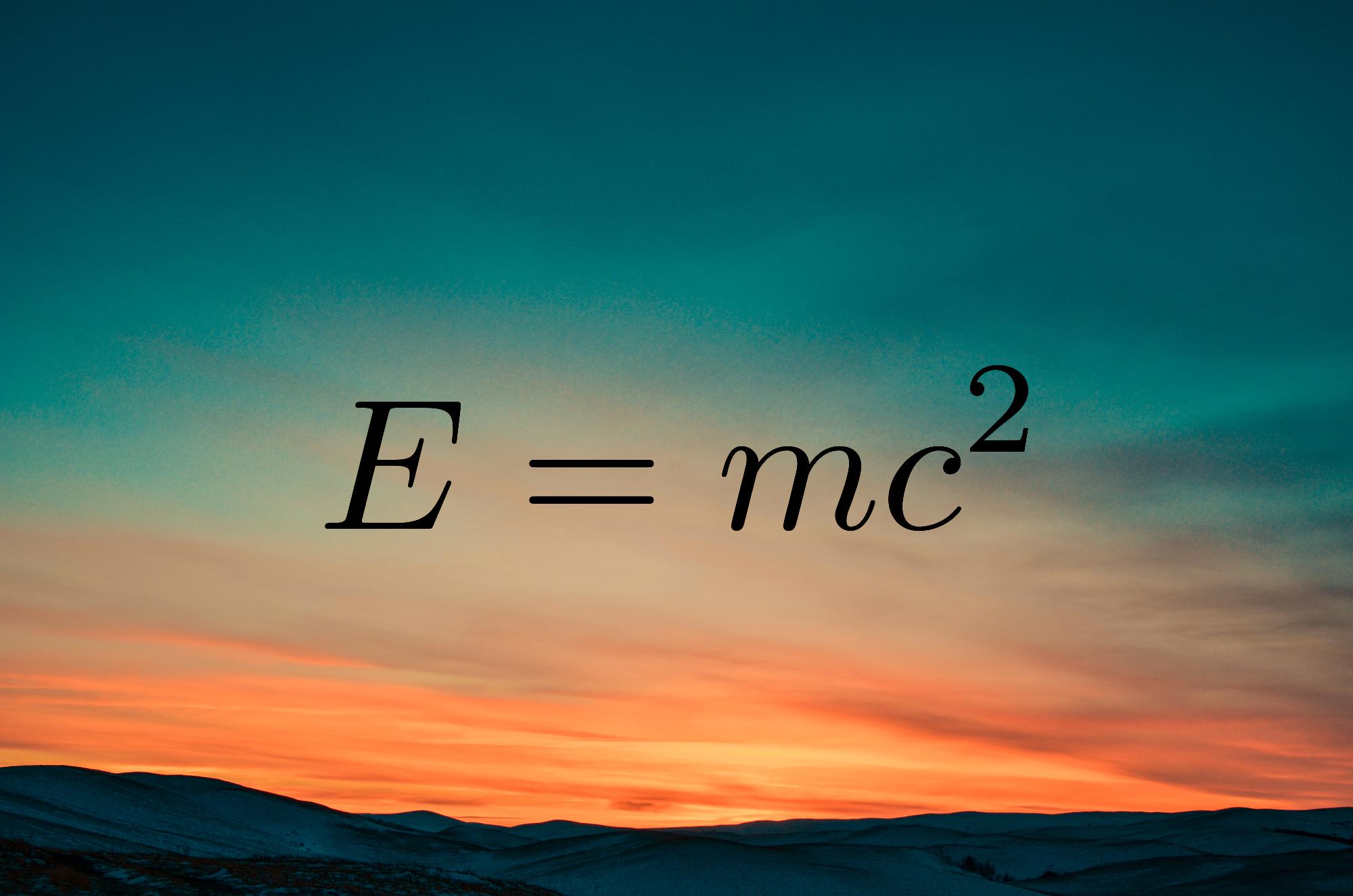
To better showcase the effects of mixed blending, see what happens below when we try to blend a blank-background text against a the textured sunset.
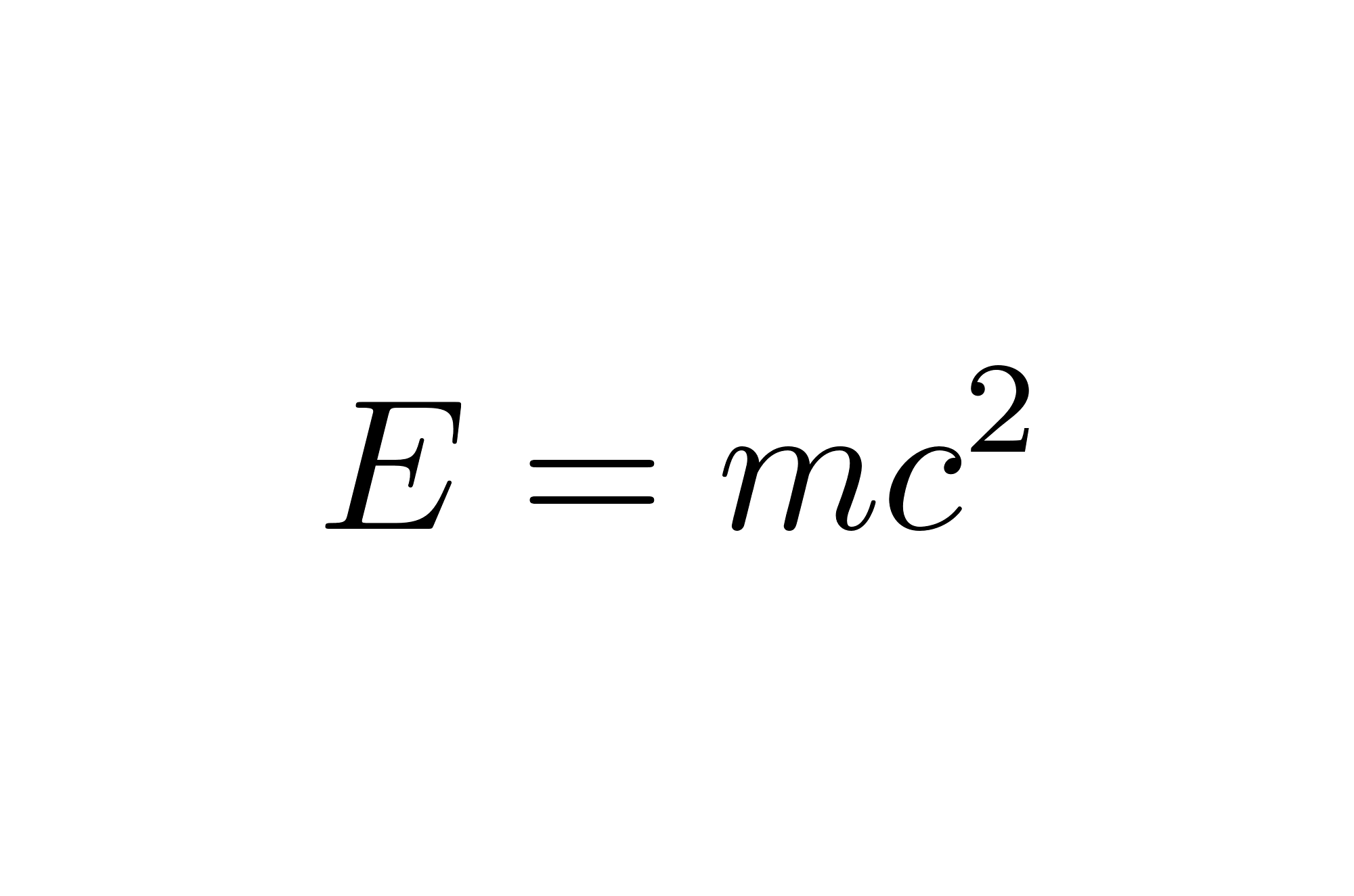
Notice that, in the case of standard Poisson blending, the smooth gradient of the background extracted from the mask are preserved and only very gradually changed. This creates the blurry impression in the Poisson blending example.
Compare this result with the mixed blend which computes the result by taking the more prominent of the two input image gradients. The sunset, which has a larger gradient than that of the white background, takes precendence over the smooth background.