Fun with Frequencies and Gradients!
CS 194-26: Image Manipulation & Computational Photography // Project 3
Emily Tsai
Part 1: Frequency Domain
1.1 Warm-Up: Sharpen Using Unsharpen
To make images look sharper, we can use the unsharp masking technique to emphasize the high frequencies of an image. First, we use a low-pass filter--in this case, the Gaussian filter--to create a blurred image containing the lower frequencies of the original image. We then subtract this image from the original image to get an image containing just the higher frequencies, or the edges. These higher frequencies are then added to the original image to add to and emphasize the distinct edges of the photo, thus creating a sharper image.

Original Image

Sharpened Image
Original Image
Low Frequencies (Gaussian)
High Frequencies = Original - Low Freq
Sharpened Image = Original + High Freq
1.2 Hybrid Images
Hybrid images are static images that change in interpretation as a function of the viewing distance. The basic idea is that high frequency (sharp edges) tends to dominate a person's perception of an image when it is available, but, at a distance, only the low frequency (smoothed) part of the signal can be seen. By blending the high frequency portion of one image with the low frequency portion of another, we get a hybrid image that leads to different interpretations at different distances.
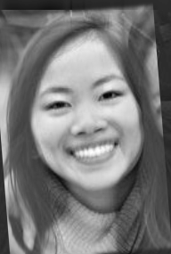
To create these images, we take two photos and then filter out the low frequencies in one photo and the high frequencies in the other photo. We then align and layer the two filtered images on top of one another; if the images are chosen and aligned correctly, we end up with a nice perspective change when we view the image first from up close and then from far away.
Derek // Nutmeg
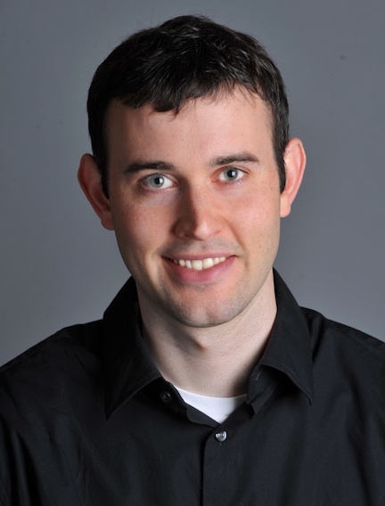
Derek
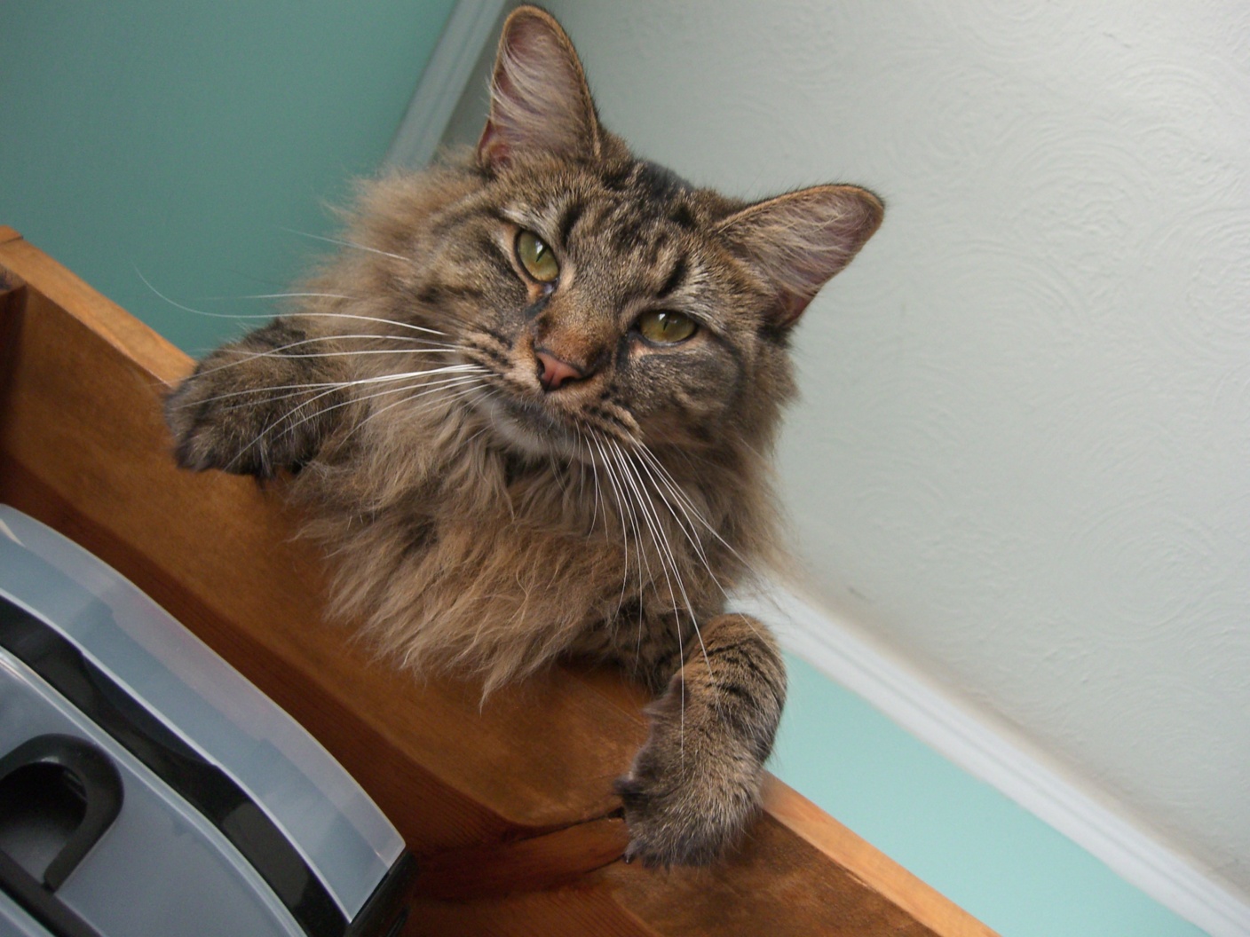
Nutmeg
Hybrid
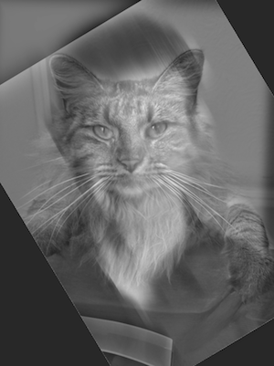
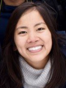
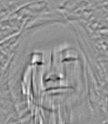
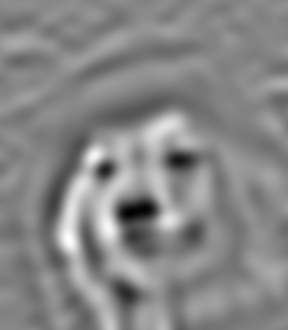
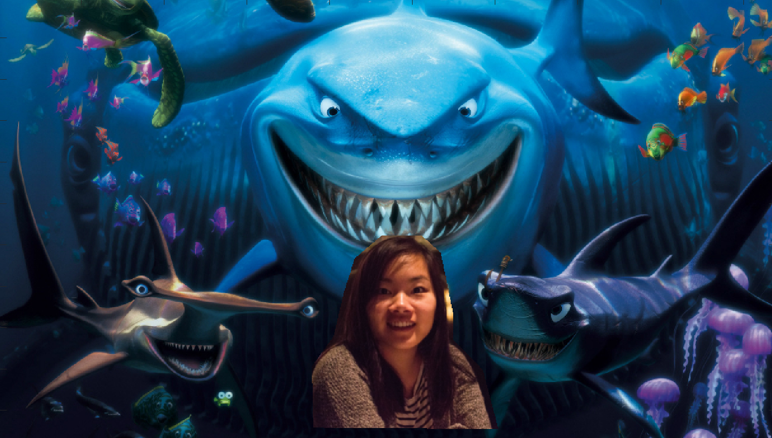
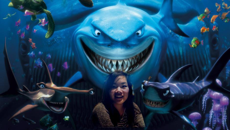
Smiling Dog // My Sister
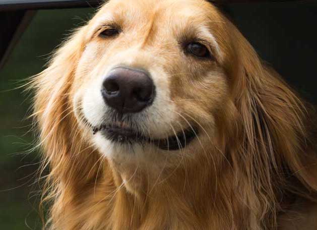
Smiling dog
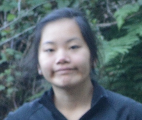
My sister

Hybrid
My Sister // Me - FAILURE
I believe this one failed because the hybrid image doesn't reveal multiple interpretations even when viewing it from different distances (apparently we look more alike than I thought). Once the faces are lined up like this, the stacked high and low frequency images don't change the interpretation of hybrid image, and it just remains a sort-of average of our faces. In addition, the sigma values chosen for this particular blend may have also contributed to this failed hybrid image as well, since the low and high frequency images look rather the same. We could possibly improve the hybrid image if we chose different sigmas that emphasized the opposite ends of the frequency spectrum more.
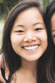
My Sister
Me
Hybrid?
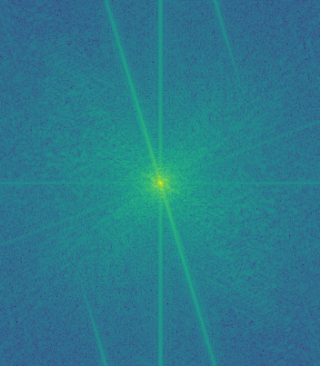
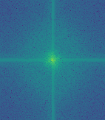
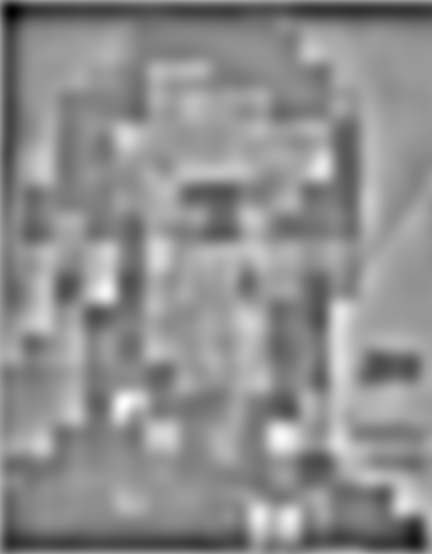
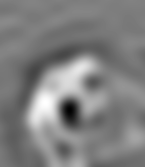
Fourier Transformations: Smiling Dog // My Sister
We can analyze and illustrate this process through frequency analysis, by showing the Fourier Transformations (FFT) of the different types of images: the two input images, the filtered (lowpass, highpass) images, and the hybrid image.
FFT of smiling dog
FFT of my sister
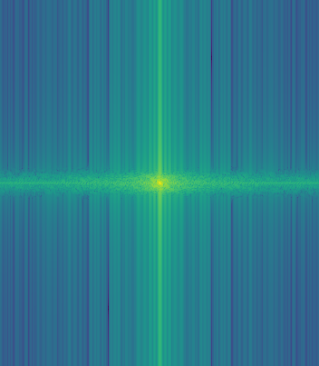
FFT of lowpass smiling dog
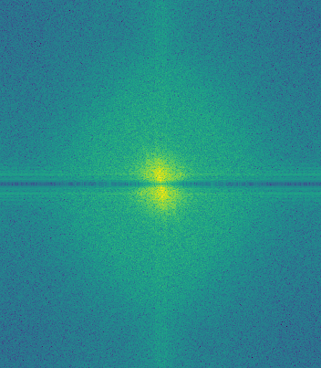
FFT of highpass my sister
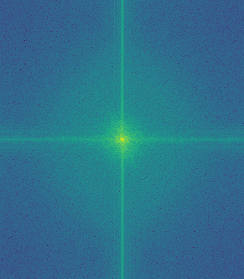
FFT of hybrid
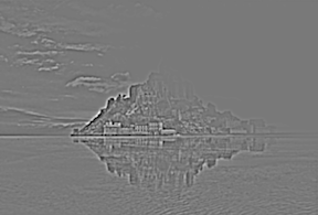
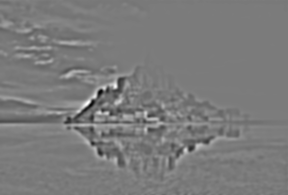
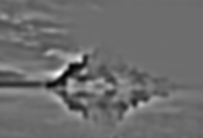
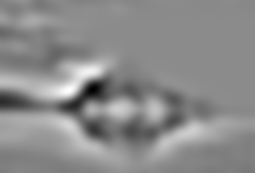
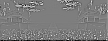
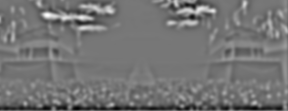
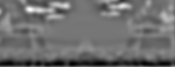
1.3 Gaussian and Laplacian Stacks
With hybrid images, either focusing on the low frequencies versus the high frequencies lets us perceive two different images. We can also use filtered stacks, which are similar to pyramids but without the downsampling, to analyze these hybrid images. Gaussian filters smooth the image, whereas Laplacian images bring out the sharper edges. After using Gaussian and Laplacian stacks to create successive layers of the Gaussian and Laplacian filter on an image, we can analyze the images at their different levels of frequencies. We can more clearly see how the lower and higher frequencies come in and out of focus as the stacks progress in their levels.
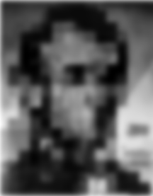
Lincoln // Gala

Gaussian: Level 1

Gaussian: Level 2
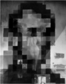
Gaussian: Level 3

Gaussian: Level 4
Gaussian: Level 5
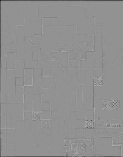
Laplacian: Level 1
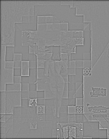
Laplacian: Level 2

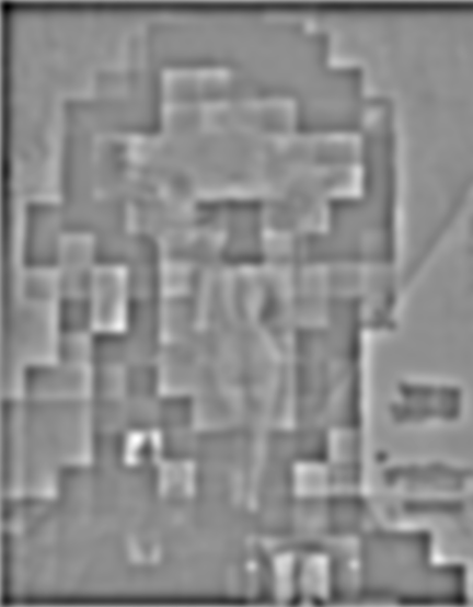
Laplacian: Level 3
Laplacian: Level 4
Laplacian: Level 5
Smiling Dog // My Sister
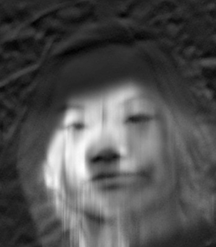
Gaussian: Level 1

Gaussian: Level 2

Gaussian: Level 3

Gaussian: Level 4
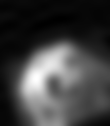
Gaussian: Level 4
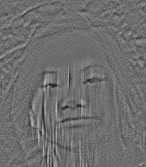
Laplacian: Level 1
Laplacian: Level 2

Laplacian: Level 3
Laplacian: Level 4
Laplacian: Level 5
1.4 Multiresolution Blending
Multiresolution blending uses Laplacian and Gaussian stacks to blend two images seamlessly along a mask. To build up a full image, we sum up the result of multiplying different levels of resolutions of a Gaussian filtered mask with different levels of resolutions of a Laplacian filtered image. The resulting image spline (the place where the two images connect) is a smooth seam that joins the two images together by gently distorting them along the mask's edge. Multiresolution blending computes this gentle seam between the two images seperately at each band of image frequencies, resulting in a much smoother, feathered seam than naive cut and paste.
Apple // Orange
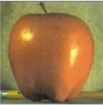
Apple
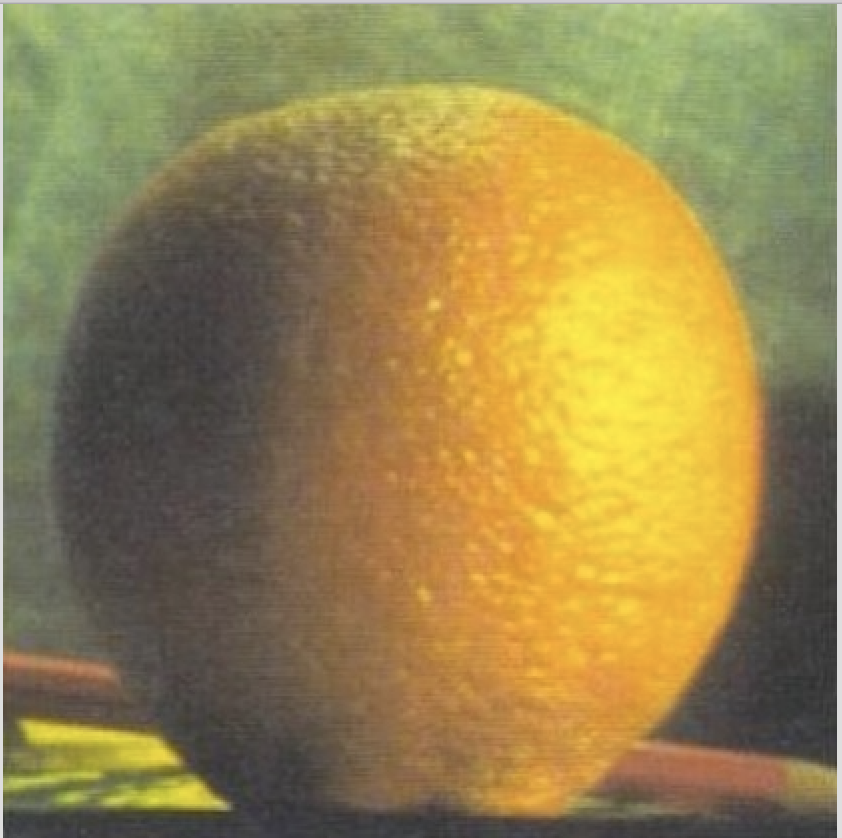
Orange
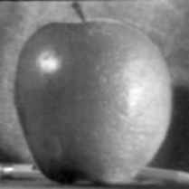
B/W Oraple
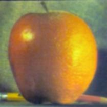
Colored Oraple
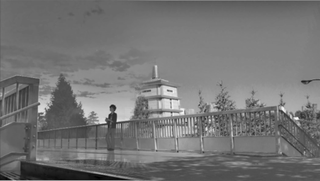
Inspired Movie Scenes
Kimi no Na wa
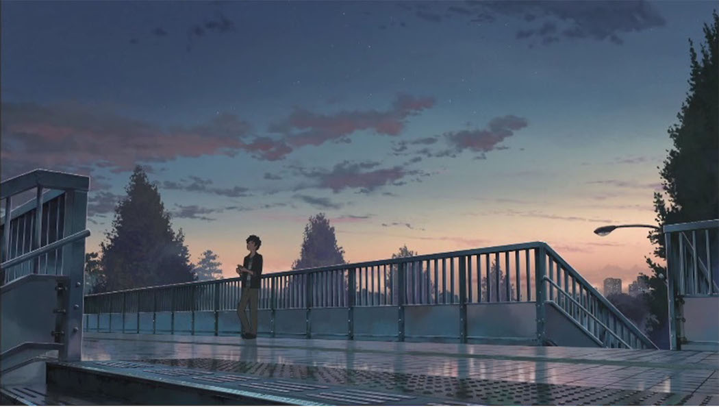
Your Name Bridge
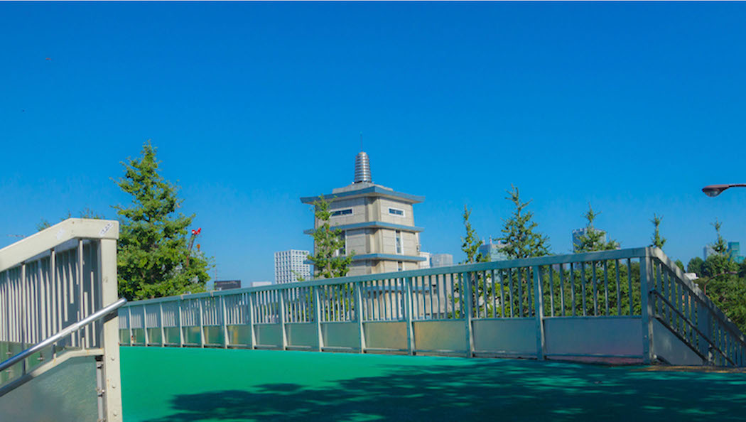
Bridge in Japan

Mask
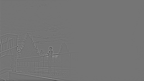
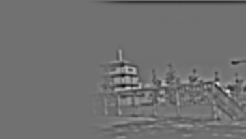
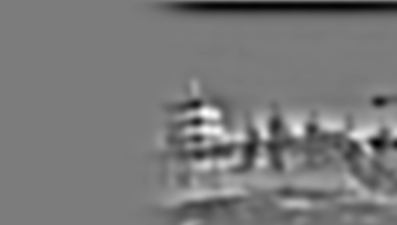
Your Name Bridge: L1
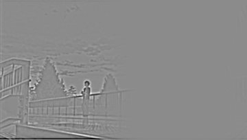
Your Name Bridge: L2
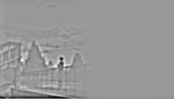
Your Name Bridge: L3
Your Name Bridge: L4
Your Name Bridge: L5

Mask
Japanese Bridge: L1
Japanese Bridge: L2
Japanese Bridge: L3
Japanese Bridge: L4
Japanese Bridge: L5
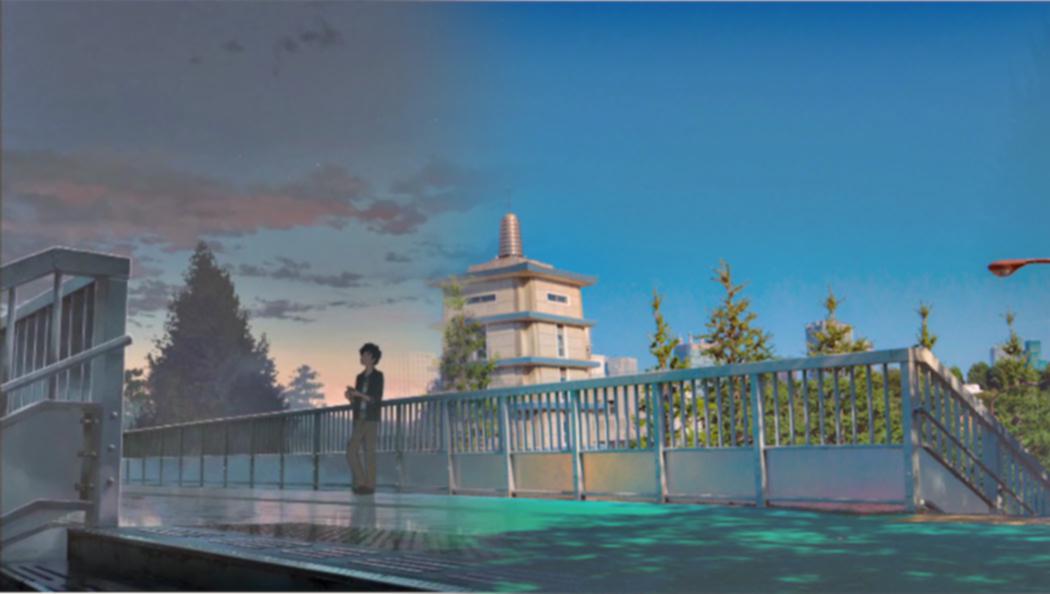
Your Name to Japanese Bridge
And the world has somehow shifted
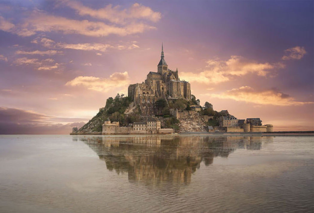
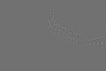
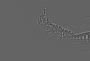
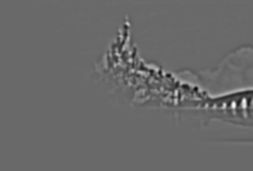
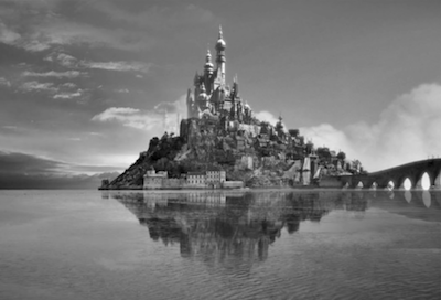
French Castle
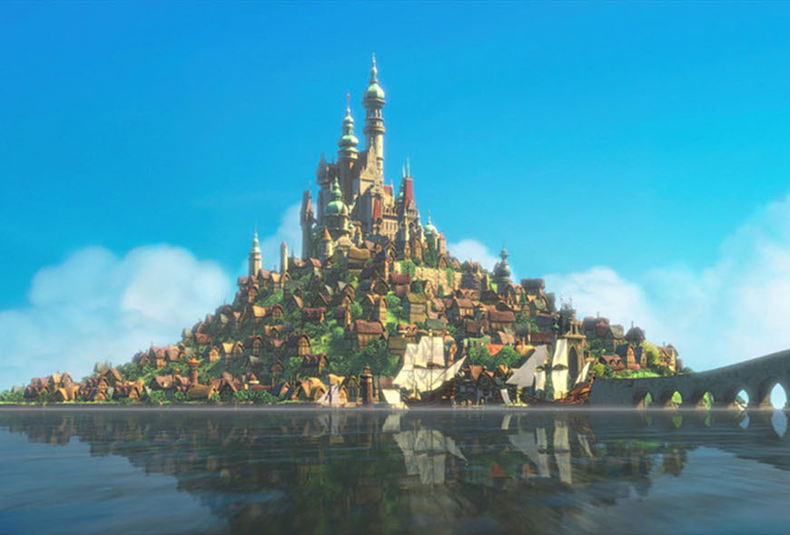
Tangled Castle
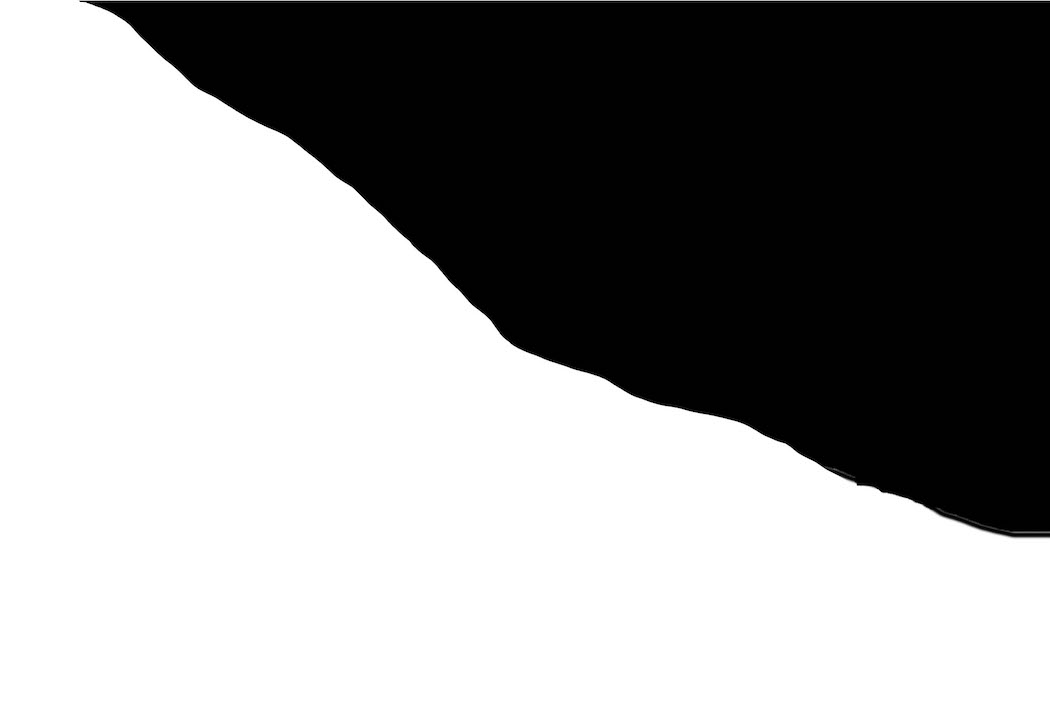
Mask
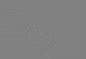
Tangled Castle: L1
Tangled Castle: L2
Tangled Castle: L3
Tangled Castle: L4
Tangled Castle: L5
Mask
French Castle: L1
French Castle: L2
French Castle: L3
French Castle: L4
French Castle: L5
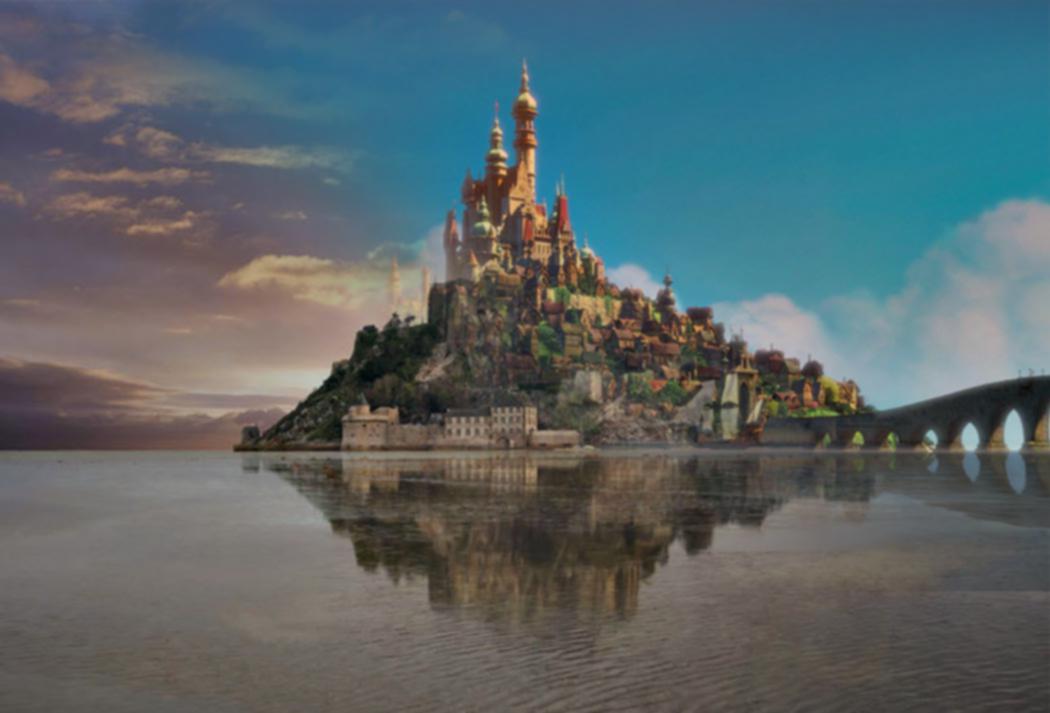
French Castle to Tangled Castle
We must be swift as the coursing river
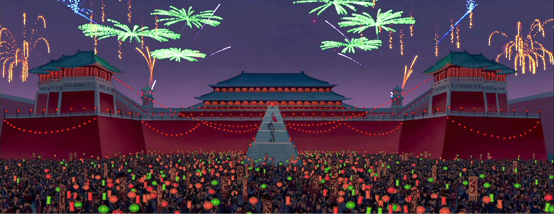
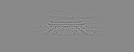
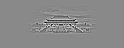
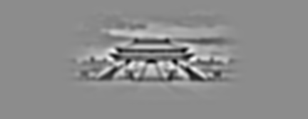
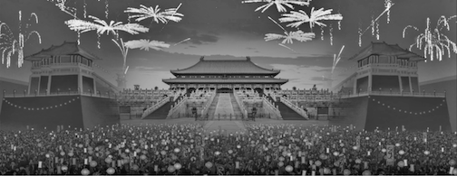
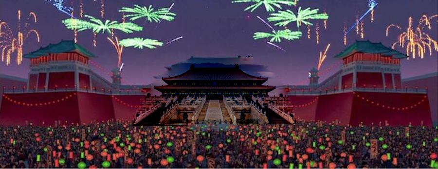
Mulan Temple
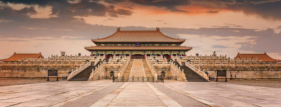
Chinese Temple
Mask
Mulan Temple: L1
Mulan Temple: L2
Mulan Temple: L3
Mulan Temple: L4
Mulan Temple: L5
Mask

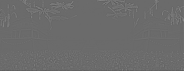
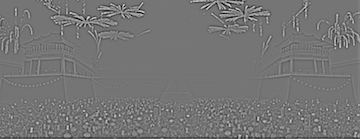
Chinese Temple: L1
Chinese Temple: L2
Chinese Temple: L3
Chinese Temple: L4

Chinese Temple: L5
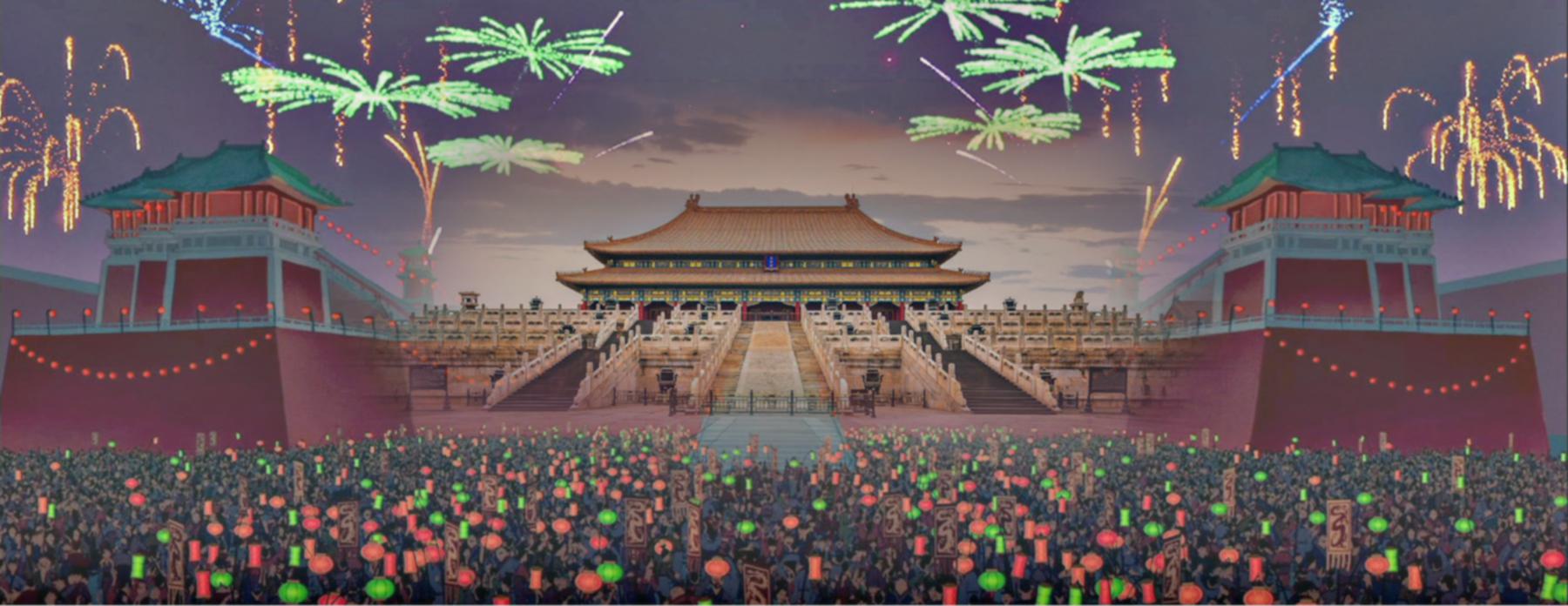
Mulan to Chinese Temple
Bells and Whistles
For some bells and whistles, I implemented the Laplacian stack blending in RGB color. The color images are shown above since they create better visual effects :-) Below are the black and white versions.
Your Name to Japanese Bridge
French Castle to Tangled Castle
Mulan to Chinese Temple
Part 2: Gradient Domain Fusion
2.1 Toy Problem
Before we begin using gradient domain fusion to blend multiple images, this toy problem gets us started on gradient domain processing by allowing us to practice working with solving a least squares problem in a matrix. In this toy example, we set up our sparse matrix of constraints, as explained in depth on the project page, which lets us recompute the pixels to reconstruct the original image. In a summary, we create a sparse matrix A of constraints, a vector b of known values, and solve for x in Ax = b.

Original Image
Reconstructed Image
2.2 Poisson Blending
This second part of the project explores Poisson gradient domain image processing, which aims to seamlessly blend an object or texture from a source image to a target background. The simplest method would be to copy and paste the pixels from one image directly into the other--but this naive implementation creates noticeable seams. However, since people often notice the gradient of an image more than the overall intensity of an image, we can set up our blending problem as finding values for the target pixels that maximally preserve the gradient of the source region without changing any of the background pixels.
Enter in: Poisson Blending
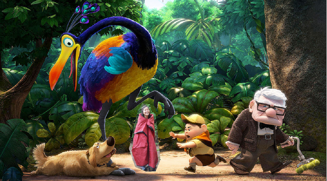
As a better method, we pick two images, a source and a target, to blend together using the gradients of the images. First, we pick a source image (the object of focus we want to combine with the target background) and a target background (the main background image onto which the source image is destined to blend with), then we create a masked region (a black and white mask of the area that outlines the source image shape) using the Matlab starter code. After we've done this, we use the least squares technique we practiced working with in the previous part to compute what pixels will make up our resulting image. To do this, we again create our sparse matrix A and known vector b; once it is set up, we divide the sparse matrix A by the vector b to get a resulting vector of pixel intensities that we reshape into our final matrix.
Each row in the sparse matrix A represents a pixel and its corresponding function that returns the output pixel. A row in matrix A is the identity function when the pixel we're considering is not in the mask. In other words, if the pixel is not going to be affected by the source image region, then the pixel will be directly copied from the target image. We do this by representing the row as an identity and storing the target pixel's value in the known vector b. Otherwise, the row in matrix A will be set up to compute the gradient of the pixel and its four neighbors from the source image. Doing so gives us the gradient that we want from the source image, and then we set it to match the intensities of its target surroundings by filling in the known values in vector b to represent these neighboring pixels' weights. The result is a source image whose masked region is integrated seamlessly into the target background.
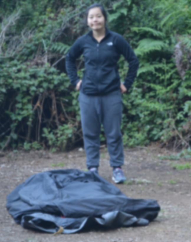
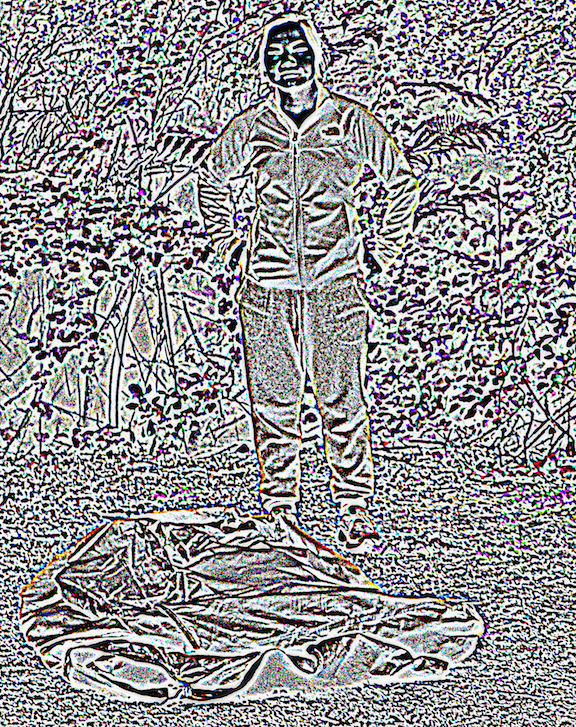
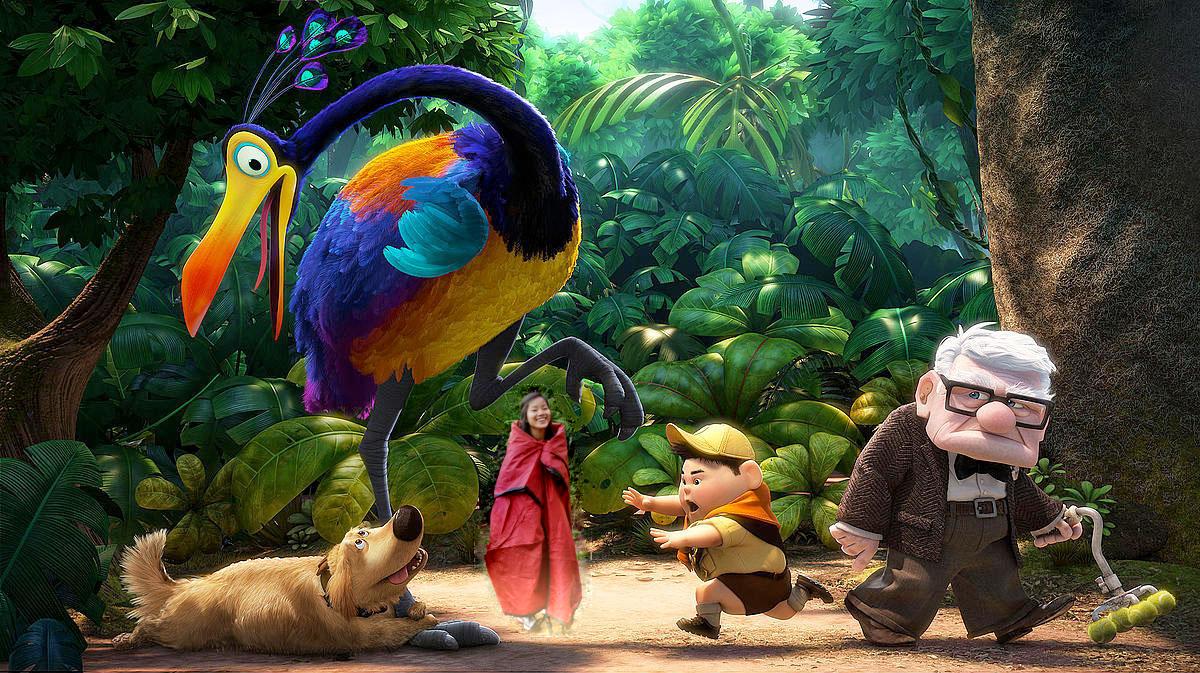
Adventures at the Campground

Target background
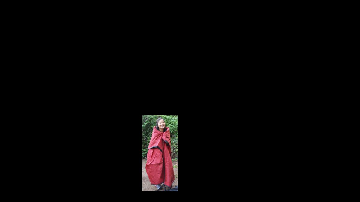
Source Image
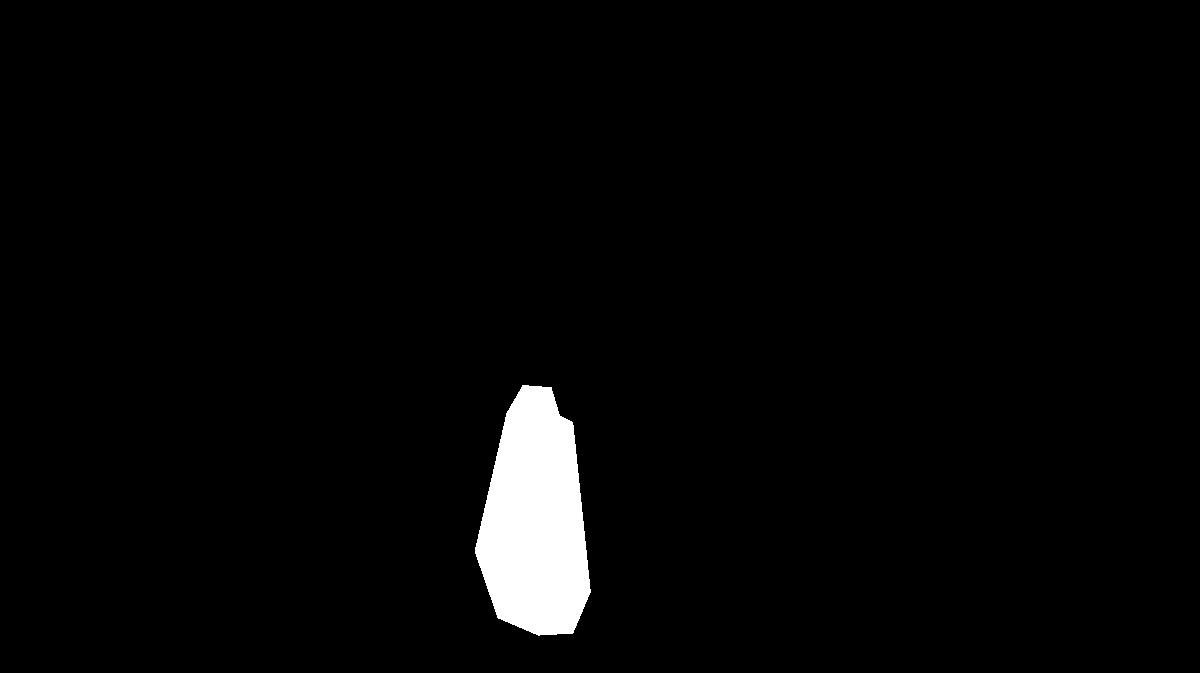
Mask Region
Naive cut, copy, and paste
My sister possibly about to get facepalmed by Kevin
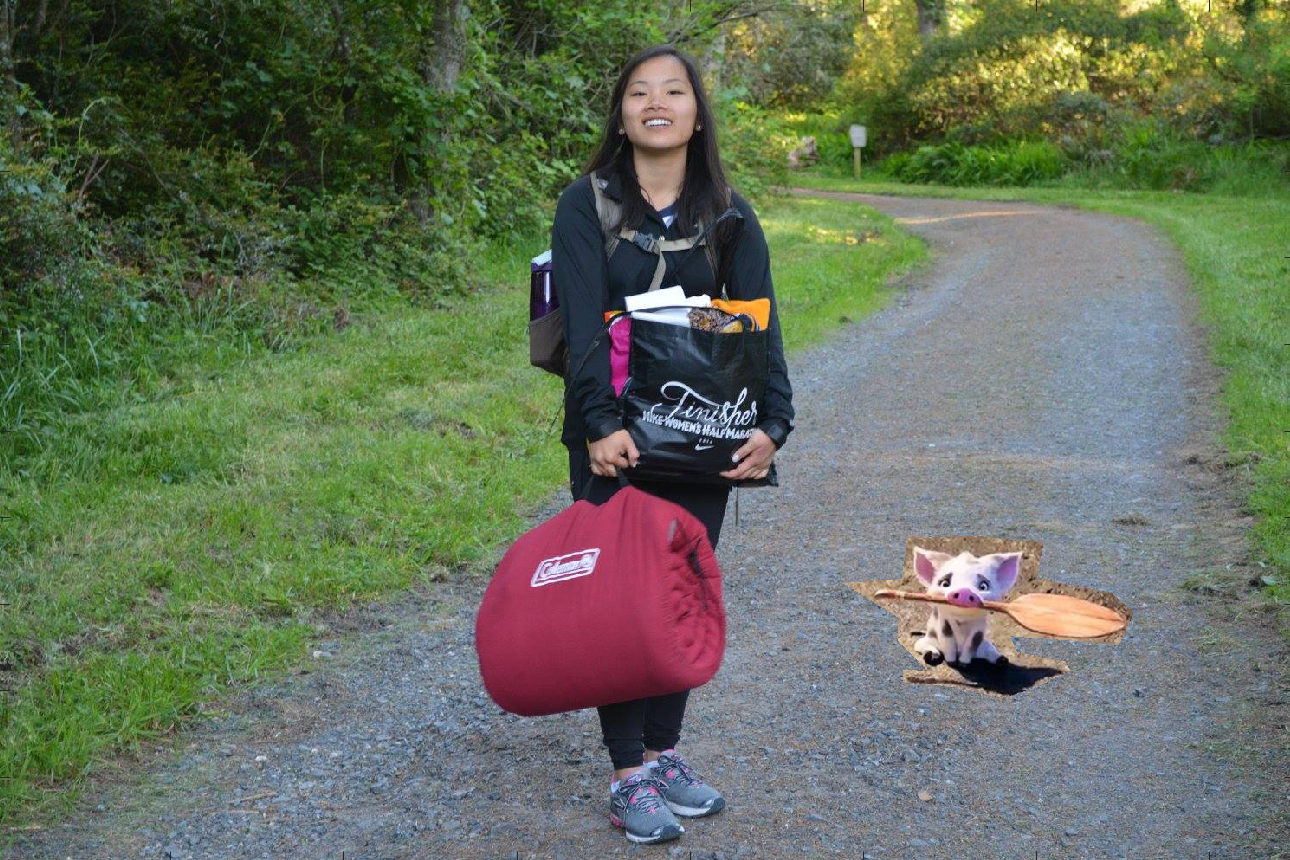
Little Helper Pua
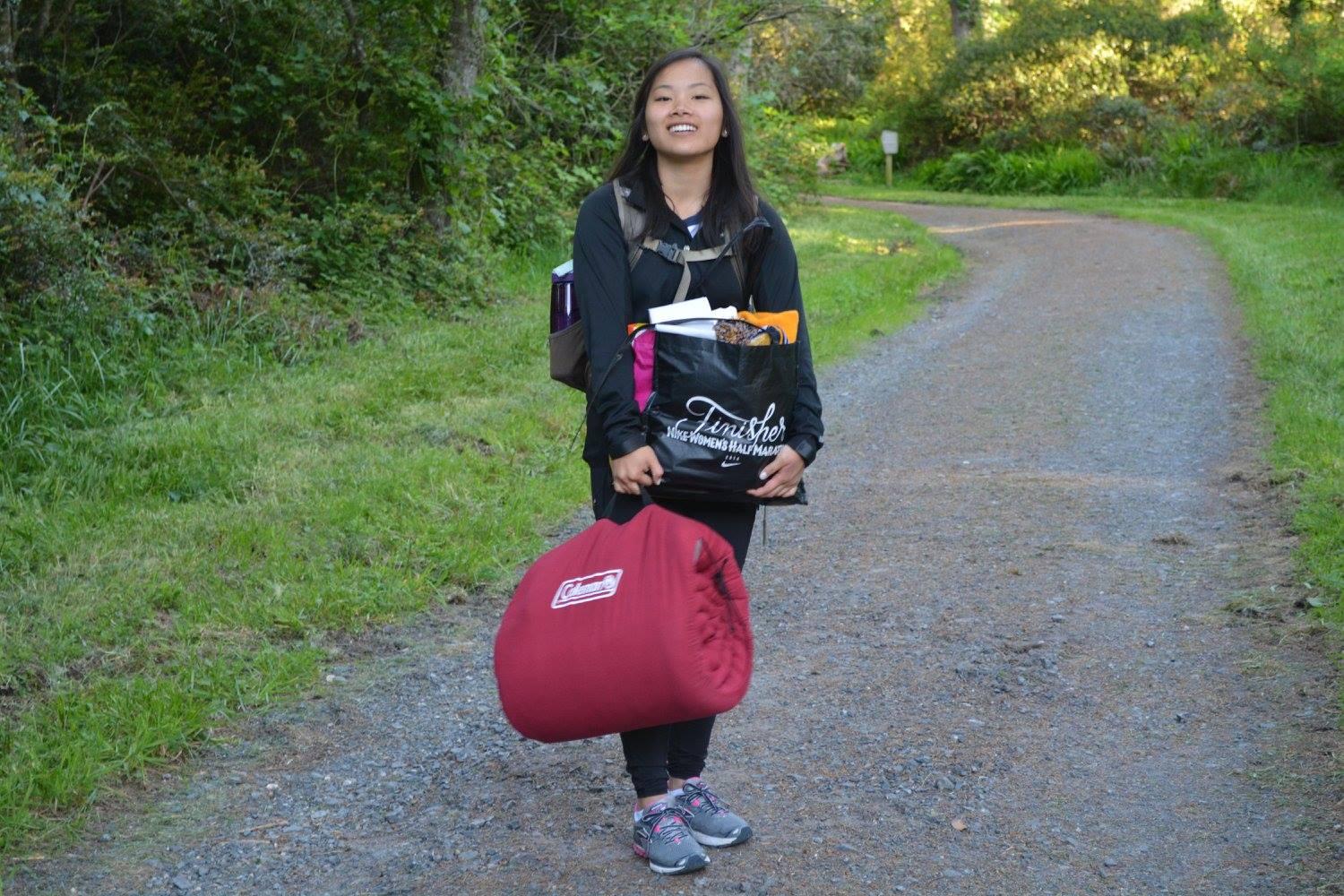
Target background
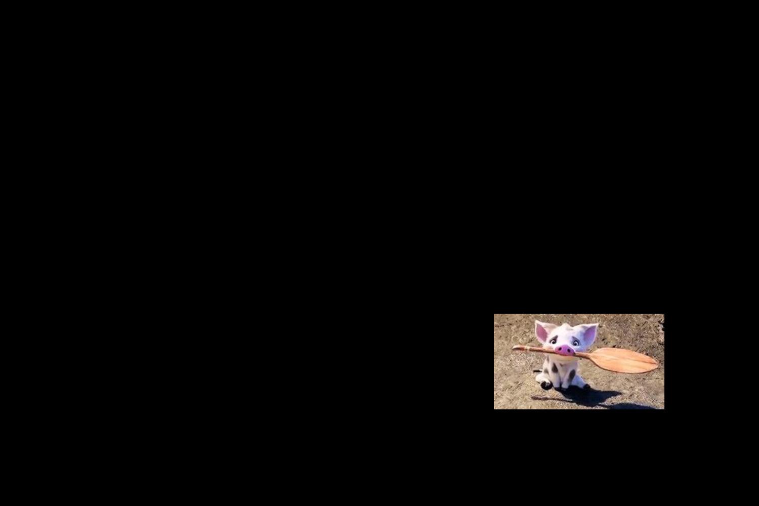
Source Image
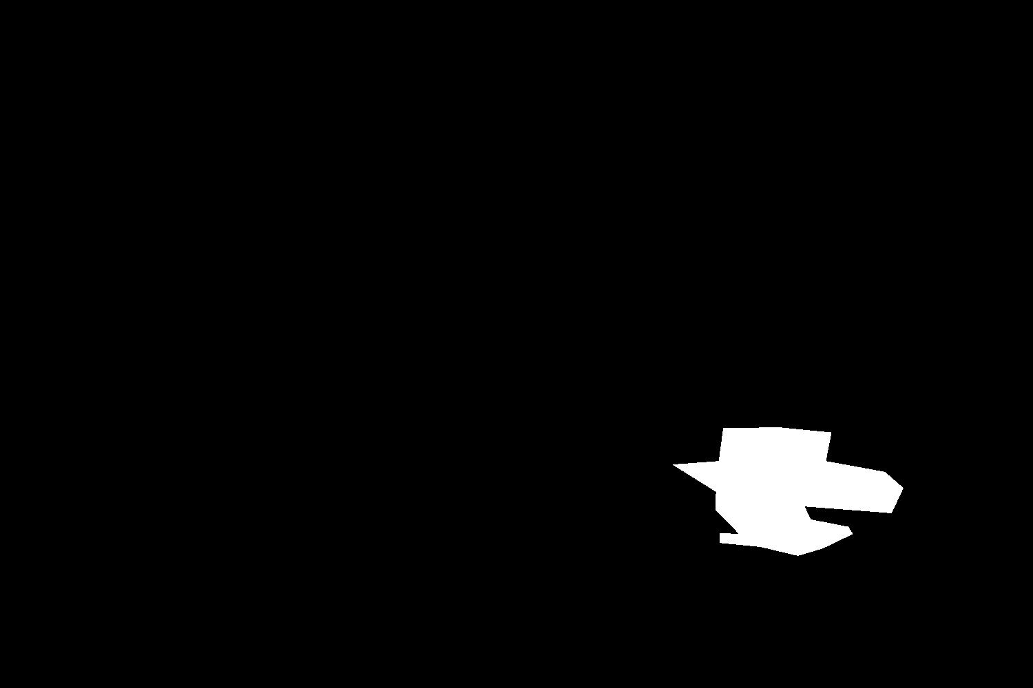
Mask Region
Naive cut, copy, and paste
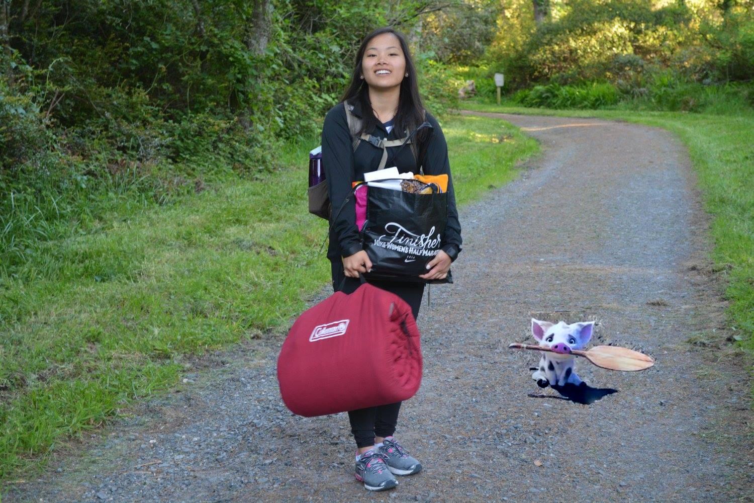
Pua helping my sister with camping supplies
Failures
Poisson blending doesn't always create the most natural-looking images, such as in this case, where the source image--in order to match its neighbors--becomes too dark and a little see-through-looking.
Simple cut and paste
Something stills seems a bit fishy here
Comparison: Laplacian Stack vs. Poisson Blending
The poisson gradient for this blend failed because the mask creator is not able to align our source image exactly with the target image--since the details are so exact to its surroundings, it doesn't make for a very good gradient domain blended image.
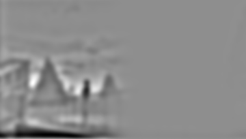
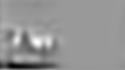
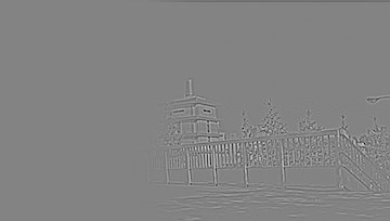
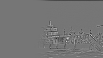
Stack: Mulan Temple // Chinese Temple
Gradient: Mulan Temple // Chinese Temple - Failed
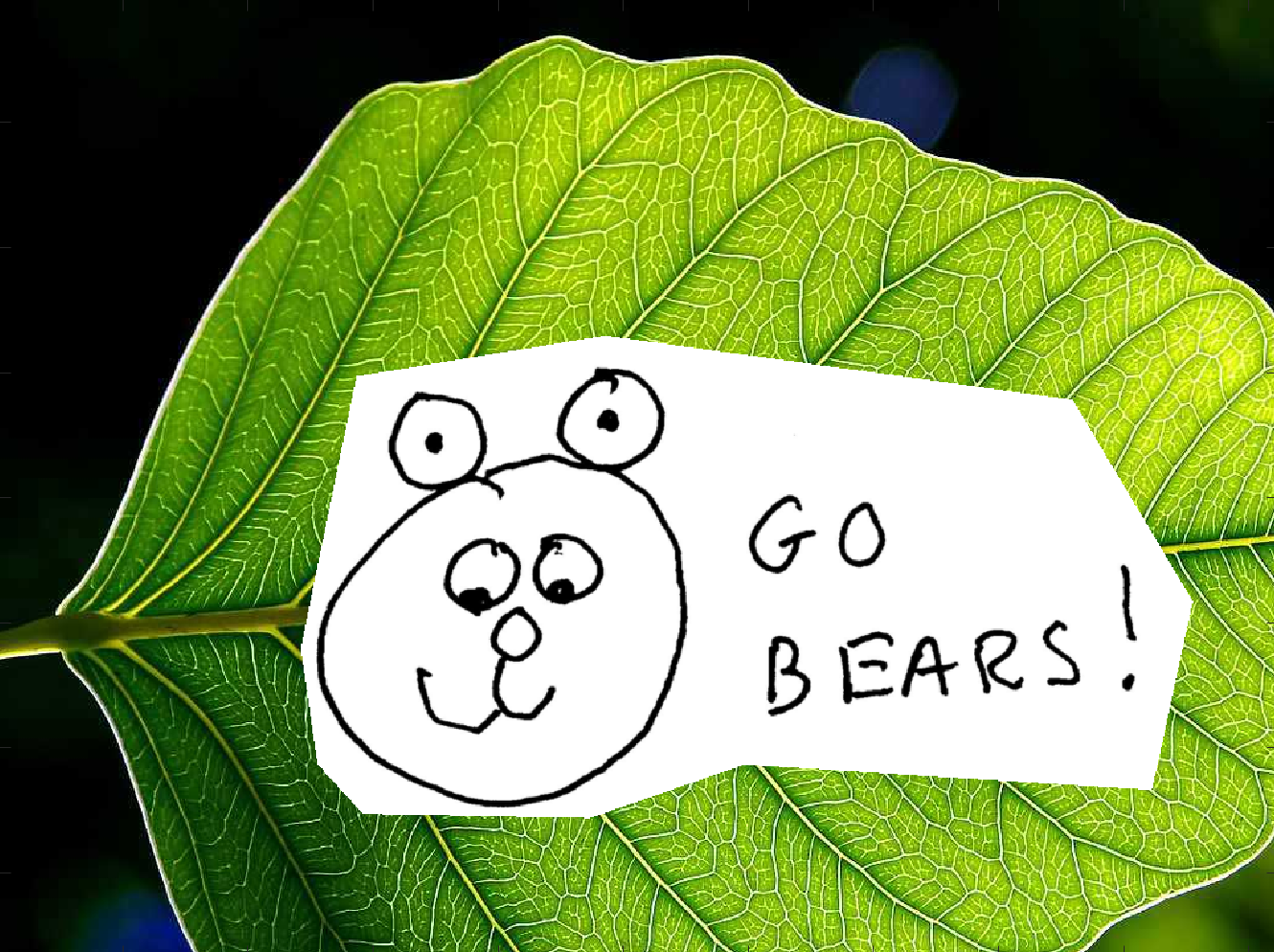
Bells and Whistles
Here we built a mixed gradient image using the value of the gradient from either the source or the target image with larger magnitude. The resulting image keeps as much detail as possible from both the source and the target images, including the leaf detailing behind the mask for the bear drawing, ince it takes the one with the larger gradient magnitude.
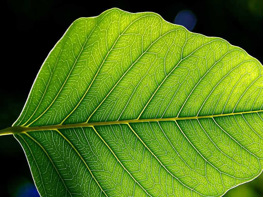
Target background
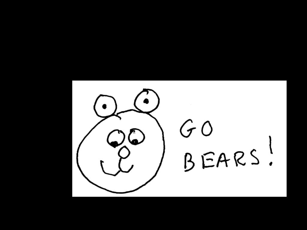
Source Image
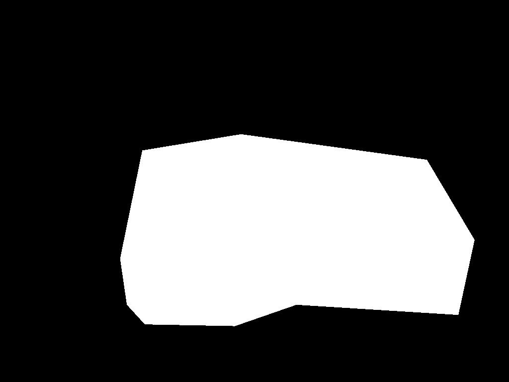
Mask Region
Normal school spirit
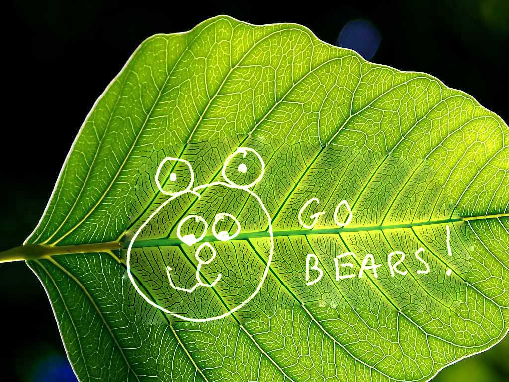
Some leafly school spirit
Parting Thoughts
I really enjoyed this project, especially the multiresolution and gradient blending! I definitely learned more about how and why matrices can be used to create these manipulations of images--which to me, used to be black-boxed. It was fun trying out different images to see which ones worked best, and rewarding when I saw how the mathematics behind it all came into play in creating these photos. It was especially cool to be able to blend drawings and real photography together to see what would happen. Thanks for stopping by to visit!