Part 1 Frequency Domain Fusion
1.1 Unsharp Masking
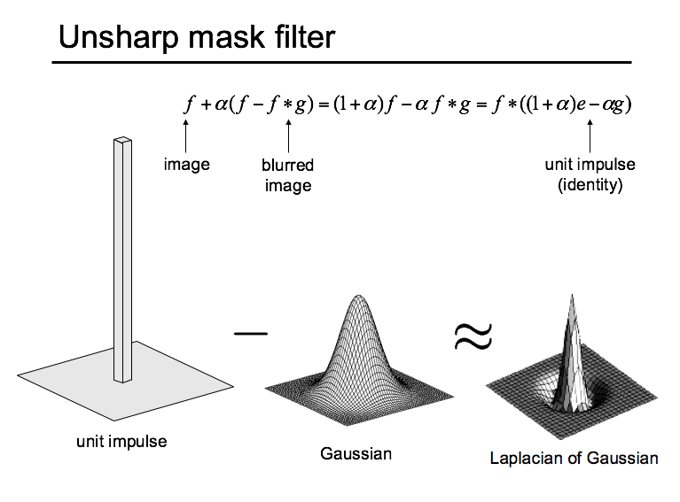
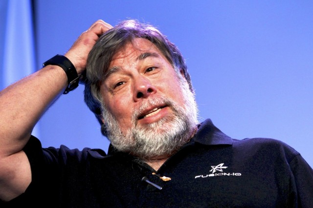
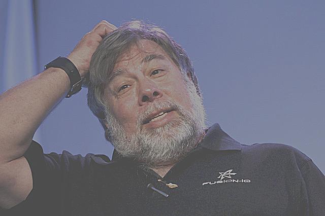
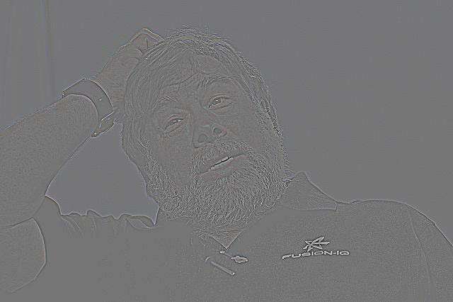
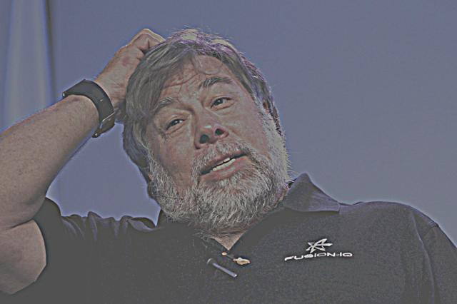
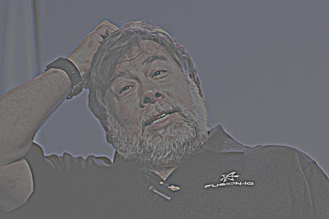
In this part, we will use unsharp masking to sharpen an image. The first image shows how unsharp masking works, and the second one is the image we want to sharpen.
 |
 |
| Unsharp Masking |
A photo of Steve Wozniak |
Now, let's play with the picture with different α and σ.
 |
 |
| α = 3, σ = 1 |
α = 100, σ = 1 |
 |
 |
| α = 3, σ = 3 |
α = 10, σ = 3 |
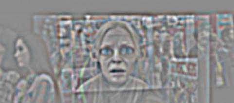
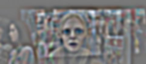
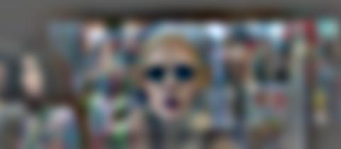
1.2 Hybrid Images
We will use the technique described in SIGGRAPH 2006
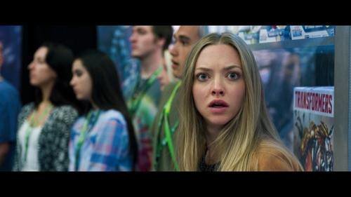
paper by Oliva, Torralba, and Schyns to hybrid several pairs of images. The general idea is to blend the high frequency portion of one image and low frequency portion of another image.
 |
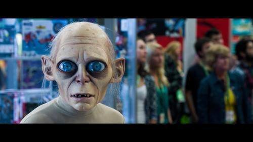 |
| Amanda Seifried |
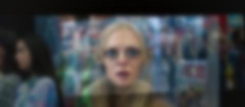
Gollum |
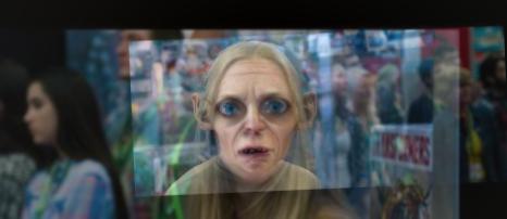 |
| Amanda Gollum |
Amanda Seifried and Gollum are quite similar to each other. Let's meet them again after Fourier transform....
 |
 |
 |
 |
 |
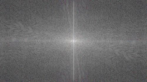
| Amanda Fourier |
Gollum Fourier |
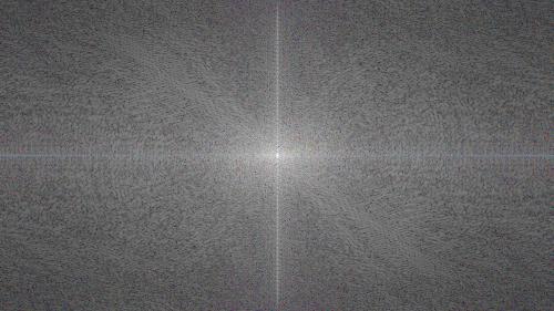
Amanda Filtered |
Gollum Filtered |
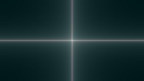
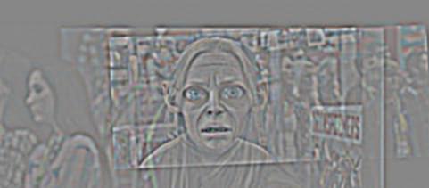
Hybrid Fourier |
 |
 |
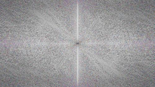
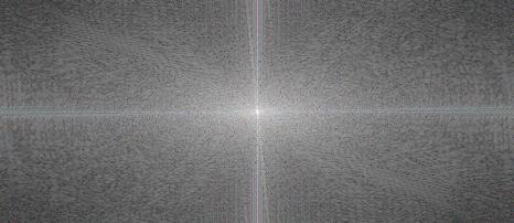
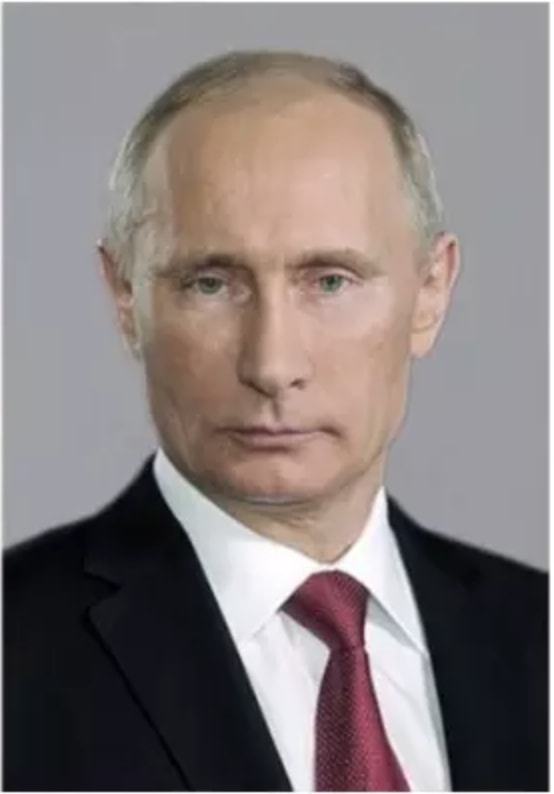
| Putin |
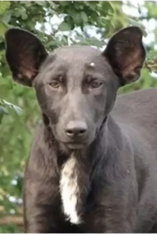
Dog |
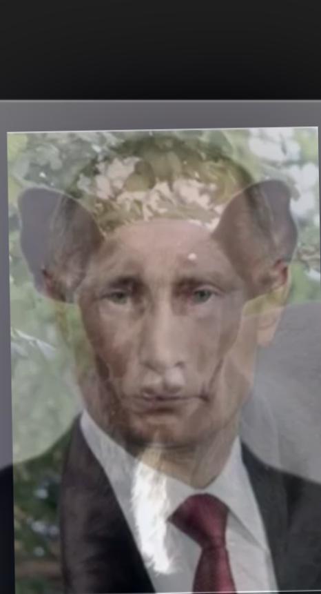 |
| Putin Dog |
So do Putin and the dog...
 |
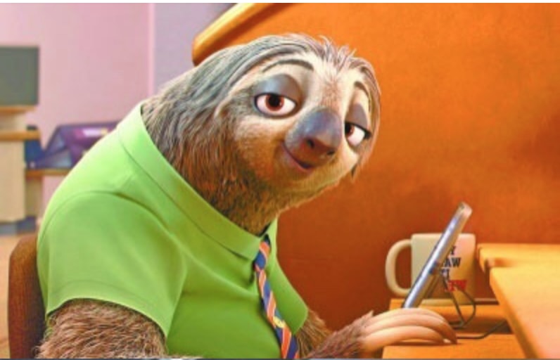 |
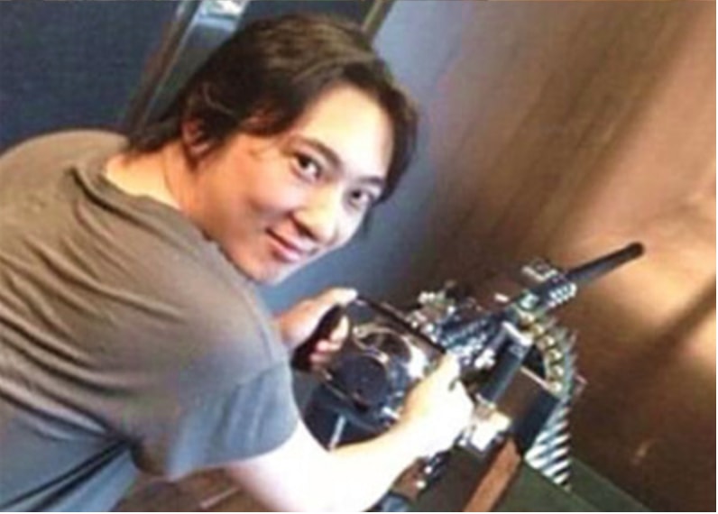
| Sicong |
Sloth |
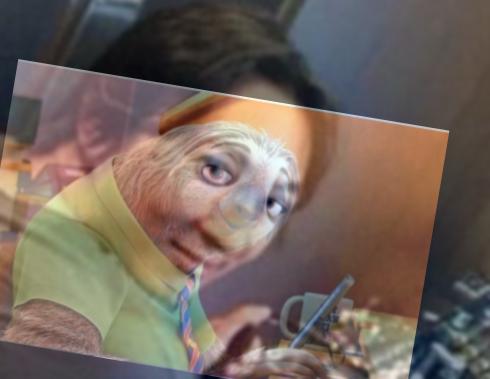 |
| Sicong Sloth |
The hybrid results of Putin dog and Amanda Gollum look good.
However, Sicong and Sloth don't match very well.
Although their eyes are aligned, the nose and mouth are too far away.
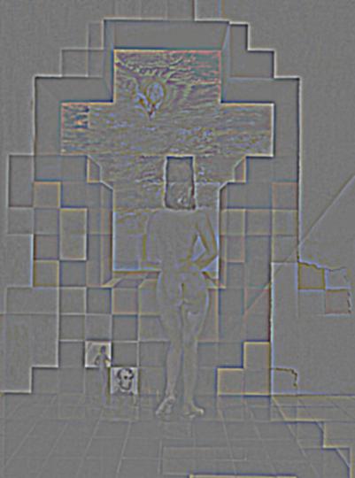
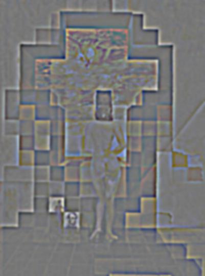
1.3 Gaussian and Laplacian Stacks
In this part, we are going to use a Gaussian stack and a Laplacian stack to analyze images.
We create the Gaussian filter at each level of the image with out downsampling to create a Gaussian stack.
Every layer of Laplacian Stack is just the difference between two Gaussian layers.
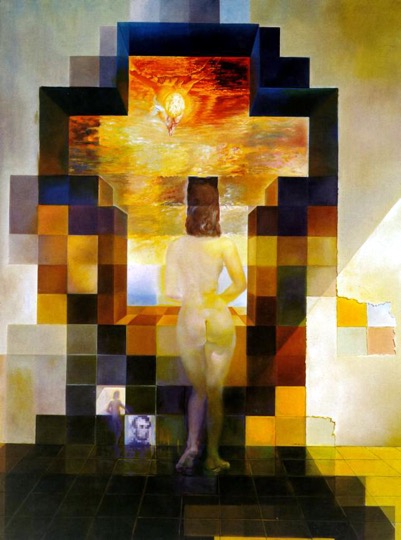 |
| Lincoln Gala |
 |
 |
 |
 |
 |
| Gaussian Layer 0 |
Gaussian Layer 1 |
Gaussian Layer 2 |
Gaussian Layer 3 |
Gaussian Layer 4 |
 |
 |
 |
 |
 |
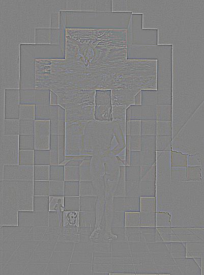
| Laplacian Layer 0 |
Laplacian Layer 1 |
Laplacian Layer 2 |
Laplacian Layer 3 |
Laplacian Layer 4 |
 |
 |
 |
 |
 |
| Gaussian Layer 0 |
Gaussian Layer 1 |
Gaussian Layer 2 |
Gaussian Layer 3 |
Gaussian Layer 4 |
 |
 |
 |
 |
 |
| Laplacian Layer 0 |
Laplacian Layer 1 |
Laplacian Layer 2 |
Laplacian Layer 3 |
Laplacian Layer 4 |
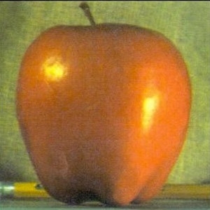
1.4 Multiresolution Blending
In this part, the goal is to blend two images seamlessly with multiresolution blending method.
Multiresolution blending computes a gentle seam between the two images seperately at each band of image frequencies,
resulting in a much smoother seam.
 |
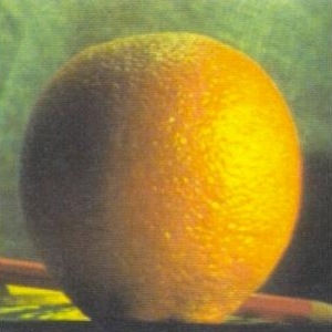 |
| Apple |
Orange |
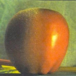 |
| Apple Orange |
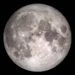
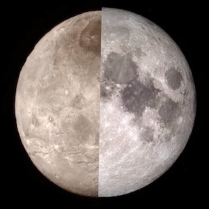
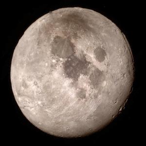
Apple Orange! Is that cool? Now let's play with moon and pluto.
 |
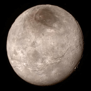 |
| Moon |
Pluto |
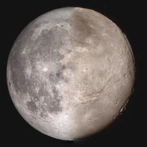 |
| Moon Pluto |
A nice combination of moon and pluto shows up.
 |
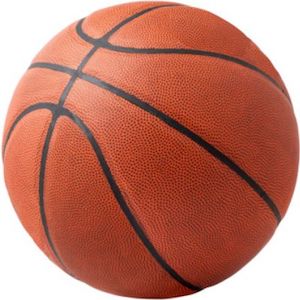 |
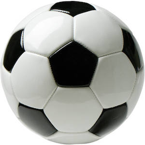
| Soccer |
Basket Ball |
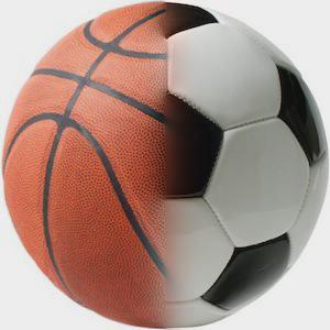 |
| Soccer Basket Ball |
An example of irregular mask, because the colors are very different.
Part 2 Gradient Domain Fusion
Second part of the project is about fusion of photos in gradient domain.
The objective of this part is to blend an object from a source image seamlessly into a target image.
The general idea is that people notice more about the gradient of an image, instead of the intensity.
So if the result image has well enough gradients, the fusion will look natural.
2.1 Toy Problem
In this example we will compute x, y gradients of an image s.
With these gradients and the pixel intensity of top left corner,
we will be able to reconstruct an image v.
We have three objectives over all.
The x-gradients of v should closely match the x-gradients of s
The y-gradients of v should closely match the y-gradients of s
The top left corners of the two images should be the same color
 |
 |
| Toy Source |
Reconstructed |
2.2 Poisson Blending
Now let's deal with Poisson Blending. The first step is to select a region in the source image,
and select a location in the target image as its bottom most blending location.
Then, we solve the following blending constraints to calculate
v.

In the end, we copy all pixels in solved
v to the target image.
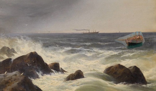
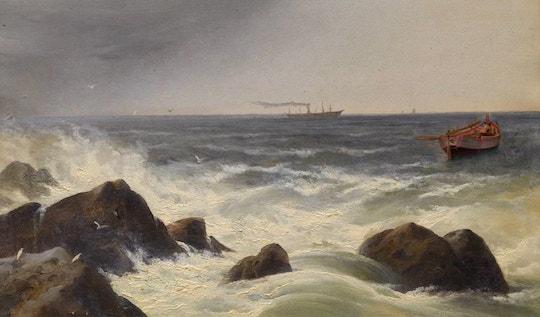
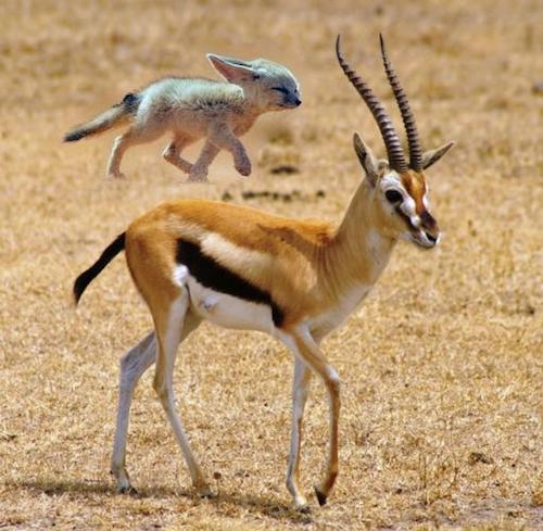
In the first example, I blend a boat into another photo.
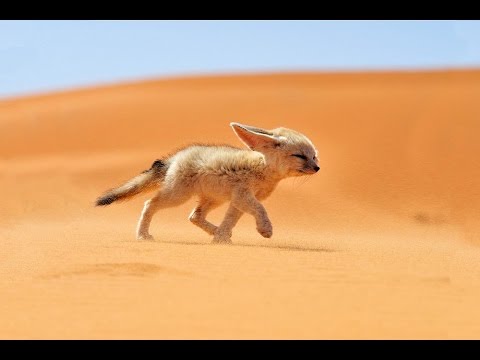
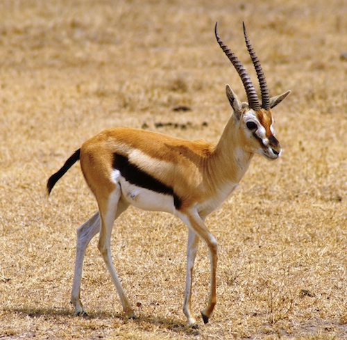
By using the technique described above, I select the fox as the object,
and the gazelle as background. After form a equation
Av = b to represent the objective function,
I use Matlab's
lscov function to solve it.
 |
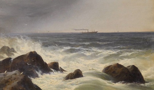 |
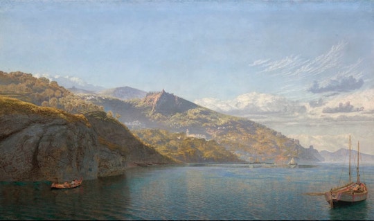
| Source Image |
Target Image |
 |
 |
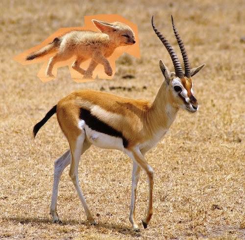
| Naive Blend |
Poisson Blend |
Then, a fox with gazelle...
 |
 |
| Source Image |
Target Image |
 |
 |
| Naive Blend |
Poisson Blend |
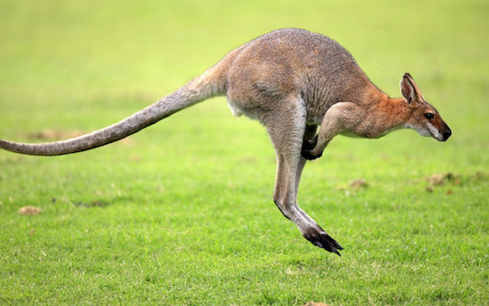
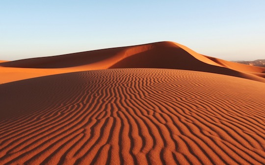
How about a kangroo in the desert?
As we can see, kangroo from first picture can't be blended well into second picture. What causes this failure?
The answer is clear, although the gradients in two picture match after blending,
the intensity of the kangroo has been changed so much that we can't ignore.
 |
 |
| Source Image |
Target Image |
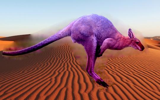 |
| Poisson Blend |
In the end, let's pick a pair of images that we blended together in part1 to deal with them with poisson blending,
and we should be able to see the difference - the result of poisson blending seems more natural in this example.
So, if we care more about gradient instead of intensity, we use poisson blending.
Otherwise, if we care more about the intensity - i.e. we want the color stay original, we use blending in frequency domain.
|
|
| Source Image |
Target Image |
|
 |
 |
| Laplacian stack Blend |
Naive Blend |
Poisson Blend |
Mixed Gradient
In this part, we will change the objective to
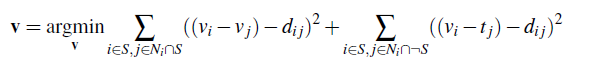
Here "d_ij" is the value of the gradient from the source or the target image with larger magnitude,
i.e. if
abs(s_i-s_j) > abs(t_i-t_j), then
d_ij = s_i-s_j; else
d_ij = t_i-t_j.
 |
 |
| Source Image |
Target Image |
 |
| Poisson Blend |