Part 1.1 - Warmup
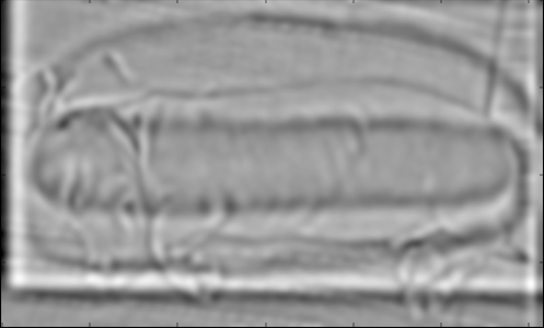
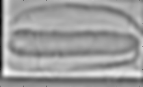
To sharpen images, I used the unsharp masking technique where Sharpened image = f + α(f − f * g).
f * g is the image convoluted with a gaussian filter using some sigma value. I used an α = 4 and sigma = 0.2
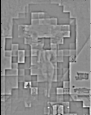
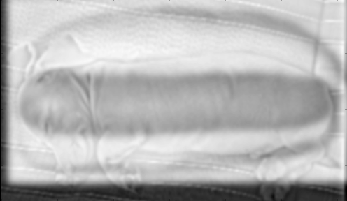
 Before sharpening
|
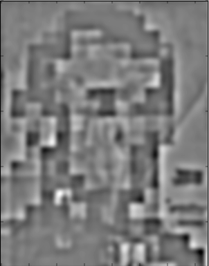
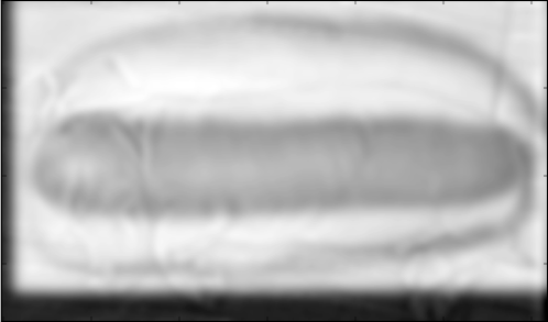
 After sharpening
|
Part 1.2 - Hybrid Images
Overview
To create hybrid images, I combined one image consisting of its low frequencies with another image consisting of its high frequencies. This method hybradizes an image because at a distance, only the low frequencies are perceived (showing image 1), and up close, the high frequencies are seen (image 2). For my favorite image (hotdog-dachshund), I used a gaussian filter with a sigma value of 3 to create a low pass filter of my first image. For the high pass filter, I used a sigma value of 3, and just subtracted from image 2 its low pass filter. Then I add the low frequency and high frequency images together.
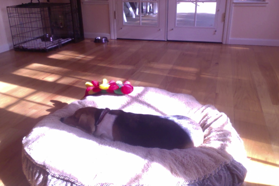
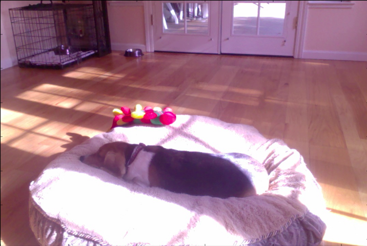
Favorite - Hot dog and Dachshund
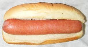 Hot dog
|
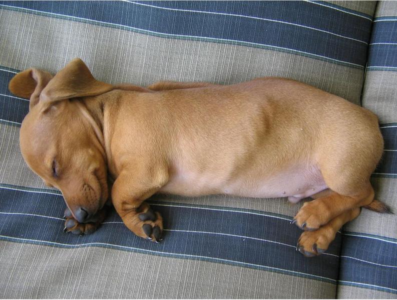 Dachshund
|
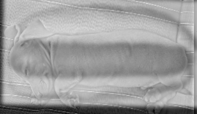 Hybrid
|
Frequency analysis of Favorite images
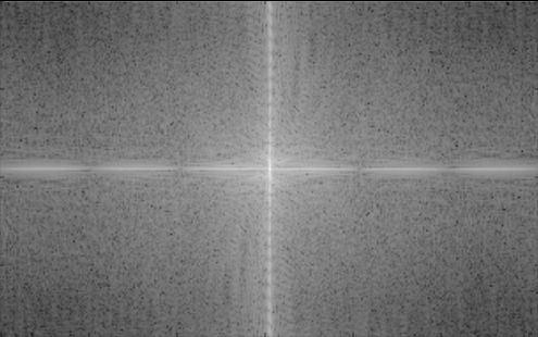 Hot dog original image
|
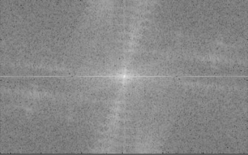 Dachshund low frequency
|
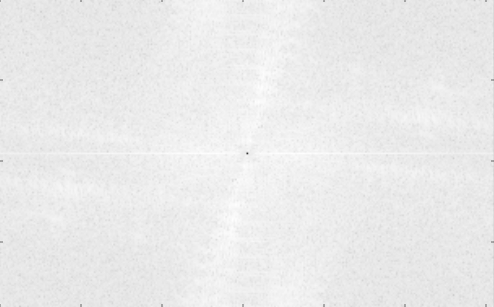 Hot dog high pass
|
 Dachshund low pass
|
 Hybrid
|
More Hybrids
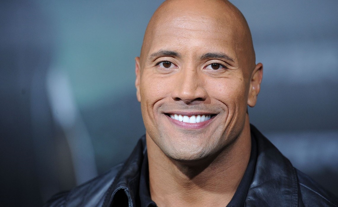 The Rock
|
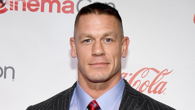 John Cena
|
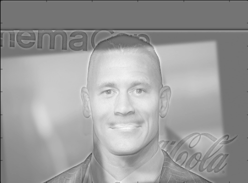 Hybrid
|
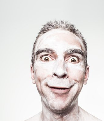 Happy face
|
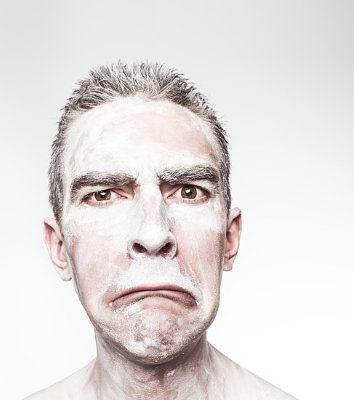 Sad face
|
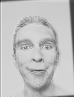 Hybrid
|
Failed attempts
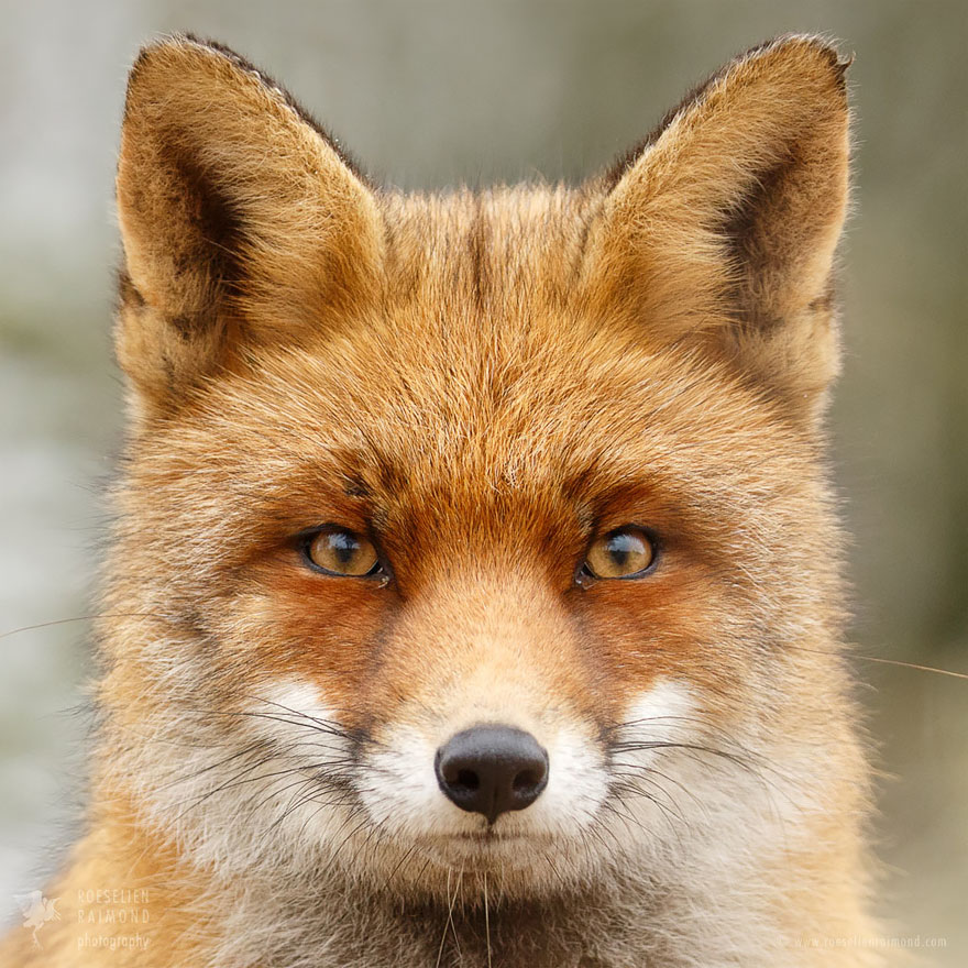 Fox
Fox
|
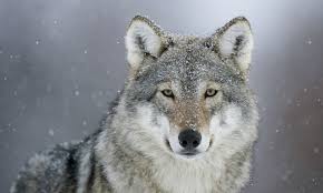 Wolf
Wolf
|
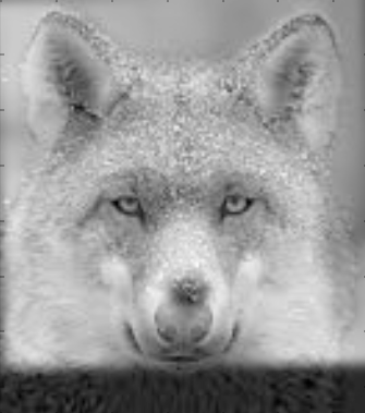 Hybrid
|
The last set of images did not align very well since there are some differences between the skeletal structures in the head (the nose of the wolf is much longer than the fox's), so even though the eyes are aligned, the rest of the head did not hybridize well.
Part 1.3 - Gaussian and Laplacian Stacks
Overview
To create the gaussian stacks, I recursively apply the gaussian filter, starting with sigma = 1, at each level of the stack, and double the sigma at each layer without downsizing the images to create a blurring effect. I created the laplacian stack by taking the difference between the current and previous layers of the gaussian stack. I also used 4 layers instead of 5, since for my favorite hybrid image, once it went to 5 layers the image was so blurry that you couldn't see anything.
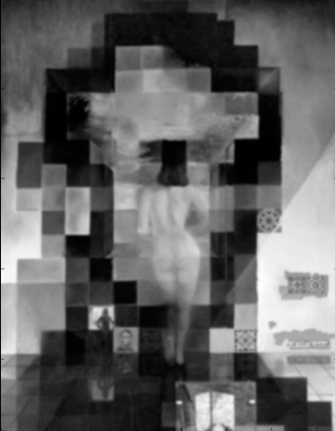
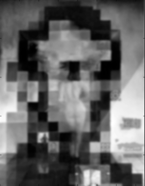
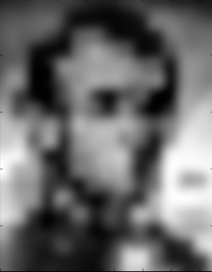
Gaussian and Laplacian stack for Lincoln and Gala painting
 Gaussian Layer 1
|
 Gaussian Layer 2
|
 Gaussian Layer 3
|
 Gaussian Layer 4
|
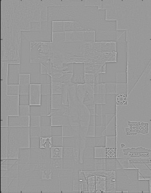 Laplacian Lincoln Layer 1
|
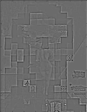 Laplacian Lincoln Layer 2
|
 Laplacian Lincoln Layer 3
|
 Laplacian Lincoln Layer 4
|
Gaussian and Laplacian stack for Hotdog-Dachshund Hybrid
 Gaussian Layer 1
|
 Gaussian Layer 2
|
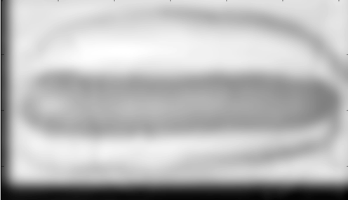 Gaussian Layer 3
|
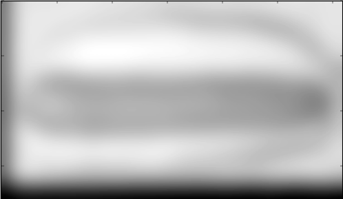 Gaussian Layer 4
|
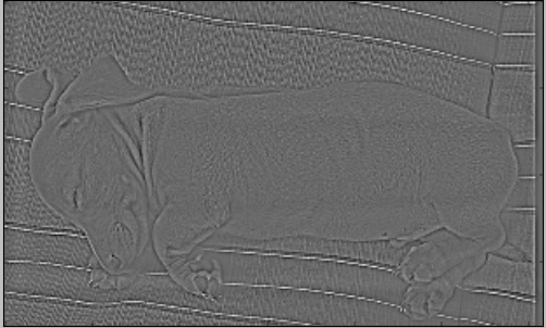 Laplacian Layer 1
|
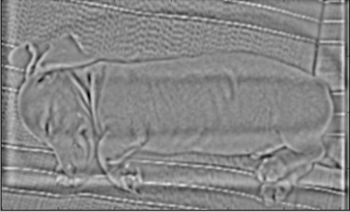 Laplacian Layer 2
|
 Laplacian Layer 3
|
 Laplacian Layer 4
|
Part 1.4 - Multiresolution Blending
Overview
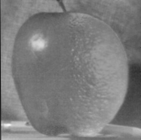
This goal of this section was to blend together two images by creating Laplacian stacks for both input images, and a Gaussian stack of the mask. For a regular blend, such as the Apple and Orange example from the paper, the mask is of the same size as the aligned images, with half of the matrix filled with 1's and the other half 0's. One of the images will appear where the 1's are while the other image appears where the 0's are. By applying a Gaussian stack of the mask, the blending becomes smoother. To combine the images, at each layer we weight each Laplacian layer with the corresponding Gaussian layer and the results like so: LS = GR*LA + (1-GR)*LB. "LS" is the combined layers, "GR" is the Gaussian mask layer, and "LA" and "LB" are the Laplacian layers for image A and B respectively. The final image is created by summing up the LS's obtained at each layer.
Split Mask
 Apple
Apple
|
 Orange
|
 OrApple
|
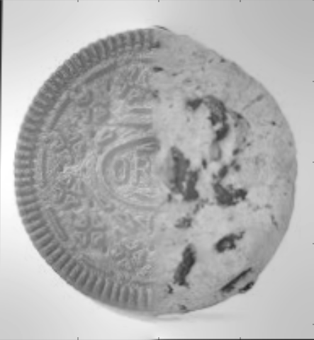
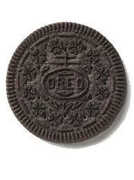 Oreo
Oreo
|
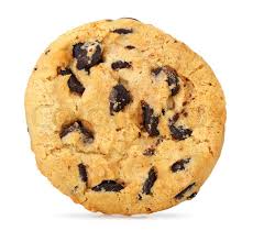 Chocolate chip cookie
|
 Chocolate chip oreo
|
For the irregular mask, I did the same calculations as the split mask (half 1's and 0's), except I provided my own mask with the 1's and 0's at the coordinates I wanted the images to show up.
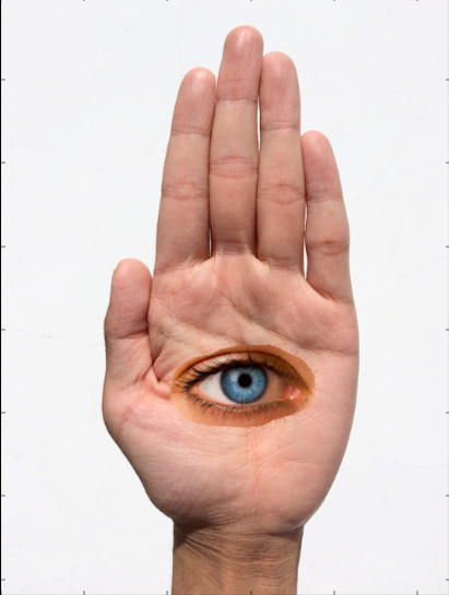
Irregular Mask
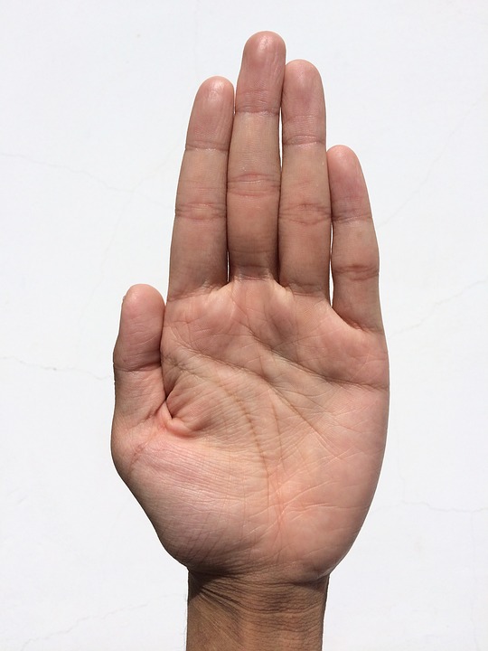 Hand
Hand
|
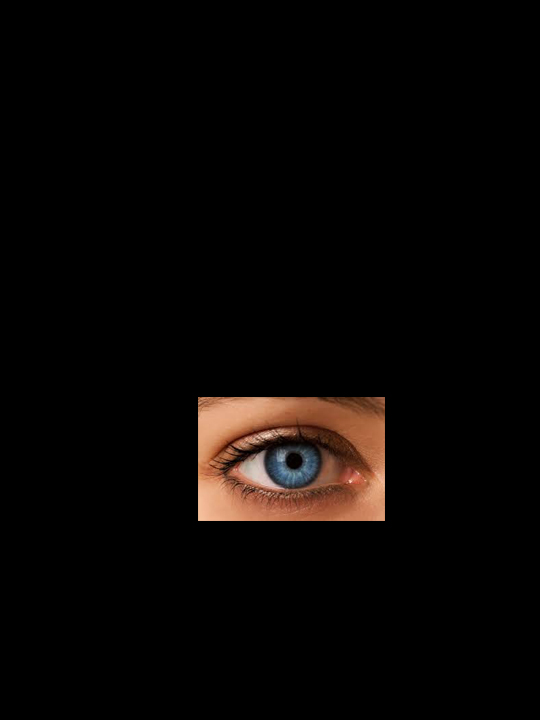 Eye
Eye
|
 Mask for eye
|
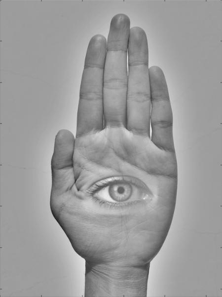 Hand-Eye
|
Part 2 - Gradient Domain Fusion
Description
Part 2 of the project explores gradient-domain processing using Poisson Blending to blend objects/textures from a source image to a target image. This insight is that gradients of an image are more noticeable to people than the overall intensity of the image, so the goal becomes finding values for the target pixels that maximally preserve the gradient of the source region without changing the pixels in the background region. We use least squares to solve for new intensity values "v" to solve the blending constraint:  .
.
That is, we want to find values "v" that minimize the gradient differences within the source image, and for pixels on the boundary of the source image, we want to minimize the gradient differences between the result and the target and the source image. This allows for a much smoother seem, while stil preserving the relationship between pixel intensities of the source image. The pixels lying outside of the source image boundary just inherit the intensity of the target image, so the background is left untouched.
Part 2.1 - Toy Problem
Overview
In the toy problem, we try to solve the constraints that the x gradients of the target should match the x gradients of the source (toy image), the y gradients of the target should match the y gradients of the source, and the top left corners of the two images should be the same color. We use least squares to solve for values "v" of the reconstructed image. The output comes out to resemble the source image quite closely, since we try to match gradients (preserve the image content) and intensity of the first pixel (preserves the overall intensity of the image).
 Original Image
|
 Reconstructed Image
|
Part 2.2 - Poisson Blending
Overview
Similarly to the toy problem, I used the previously mentioned equation to find values "v" that minimized gradients, but in this case I tried to minimize gradients in the 4 NSEW directions. And since these are color images, I just computed least squares on all the color channels of the source and target, and then stacked the results to form the final picture. I supplied my own source and mask images using similar techniques to the irregular mask for 1.4. Below, I've shown my favorite blending of a bathtub and a shark. For comparison, I've also shown a naive copy-paste of the source pixels onto the target pixels. In the naive case, the seam is very apparent since we do nothing to match the gradients, and the intensity of both images are unaltered. However, with poisson blending, we minimize the gradient between the blended image and target image, and we also try to preserve the gradient within the source image. This causes the overall intensity of the source to match with the target, so the water from the shark image matches more with the water in the bathtub, and the color of the shark is lightened to reflect the new water image.
Favorite Blending Result
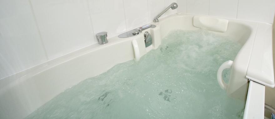 Bathtub Target Image
|
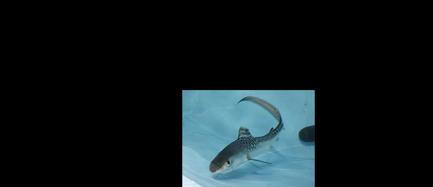 Shark Source Image
|
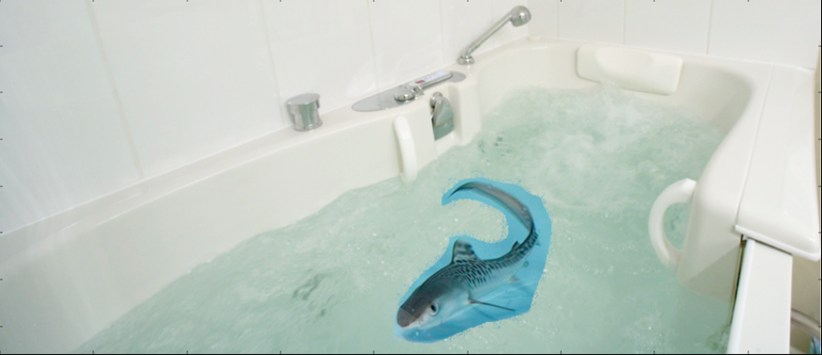 Source Pixels Copied onto Target
|
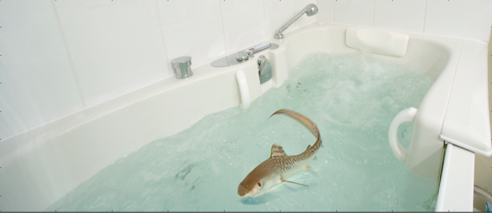 Poisson Blending of Source and Target
|
Other Blending Results
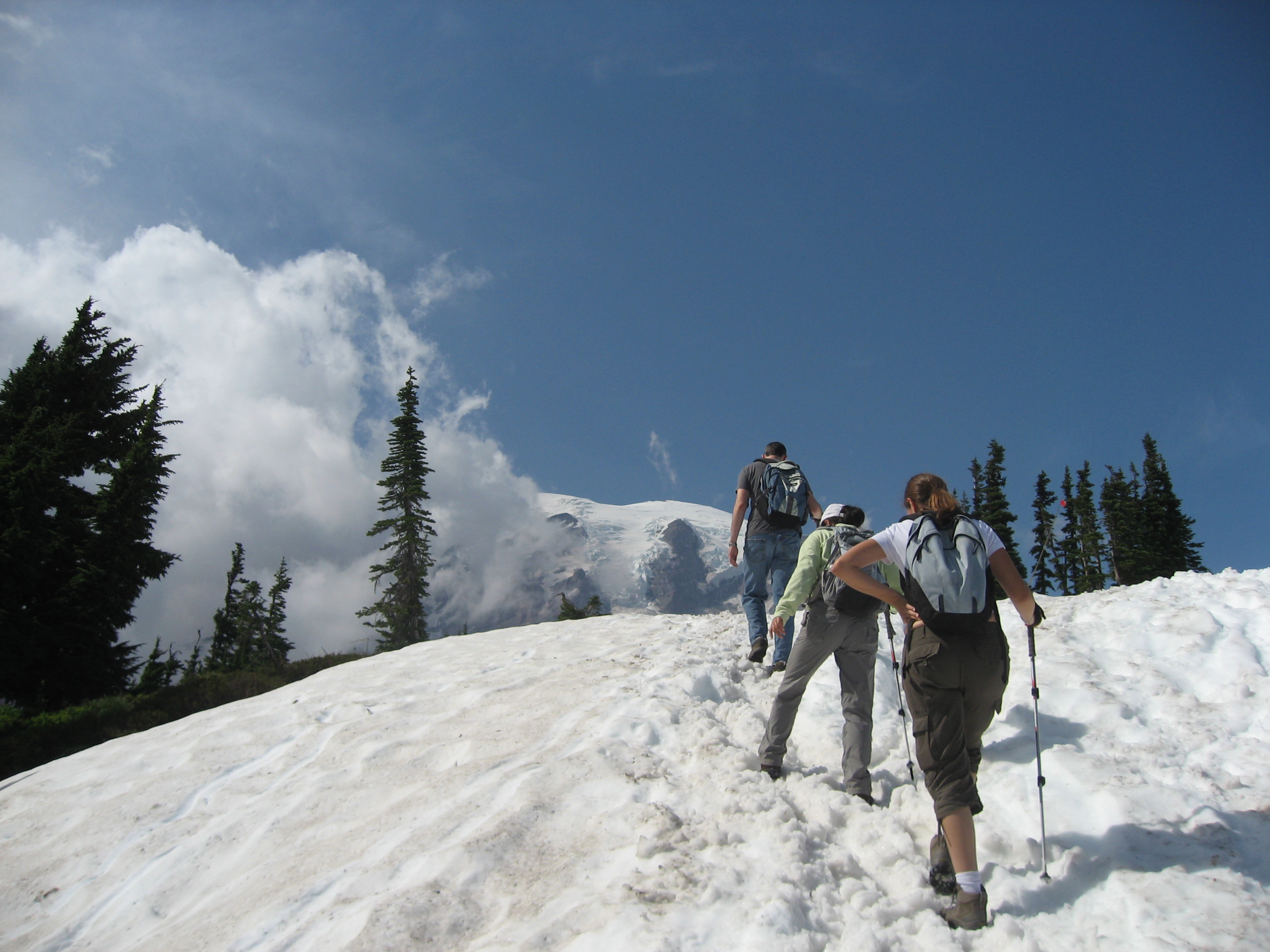 Snowy Mountain Target Image
|
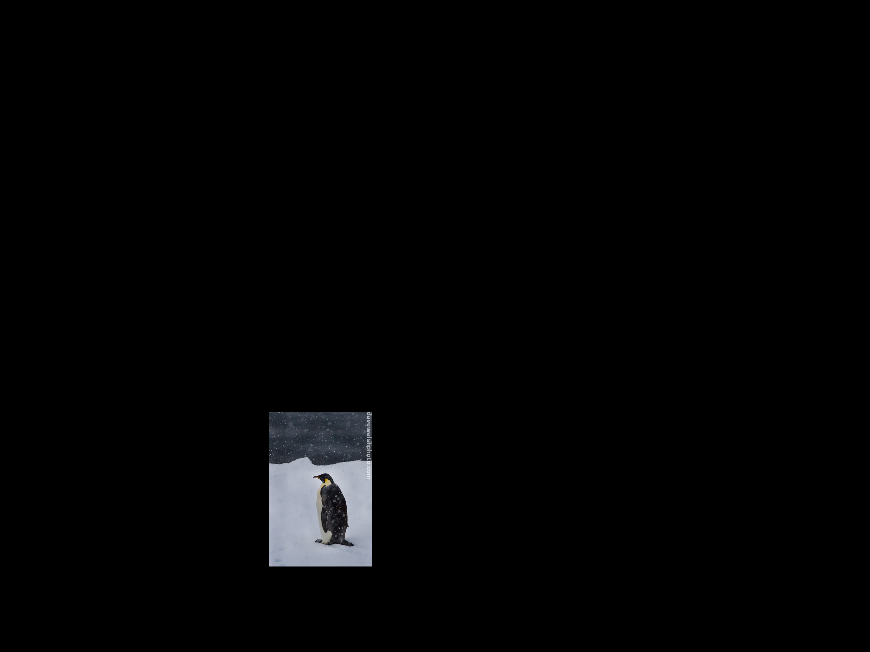 Penguin Source Image
|
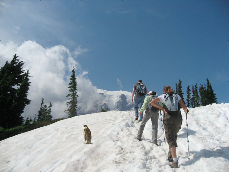 Poisson Blend
|
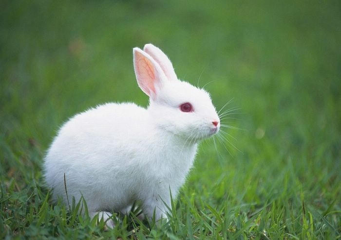 Rabbit Target Image
|
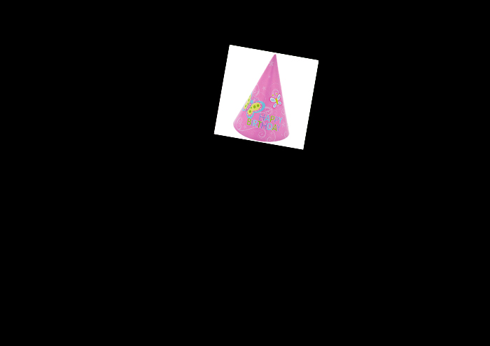 Party Hat Source Image
|
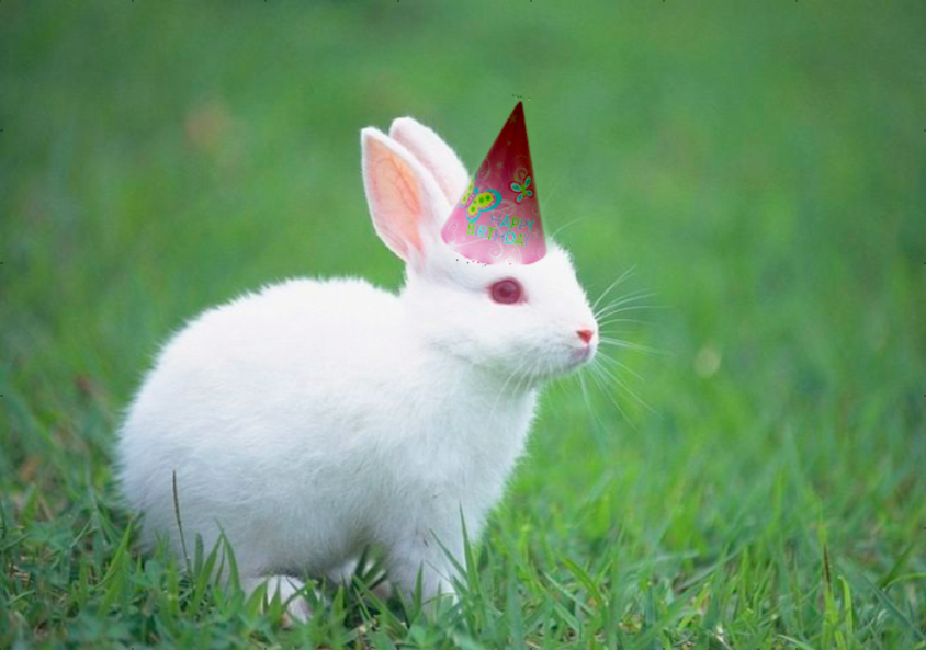 Poisson Blend
|
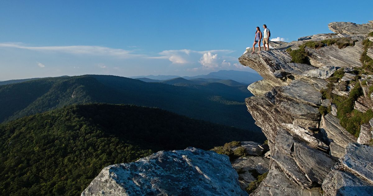 Mountain Target Image
|
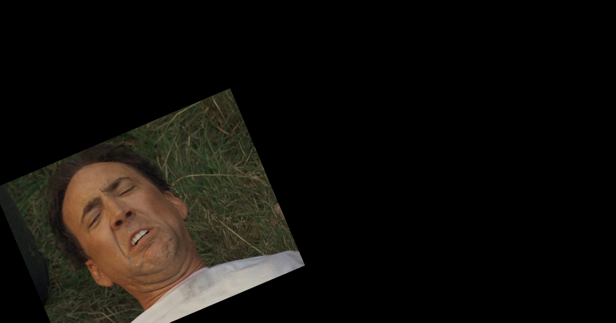 Nicholas Cage Source Image
|
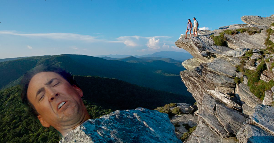 Poisson Blend
|
After computing least squares, I tried to normalize the result vector to be within values of (0, 255). This is because after computing least squares, the values might lie outside of this range, causing some awkward coloring (like the below failed image).
Failed Attempt
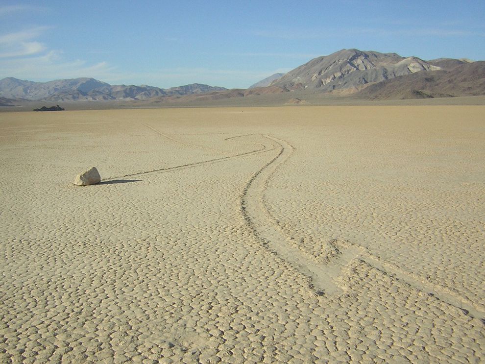 Desert Target Image
|
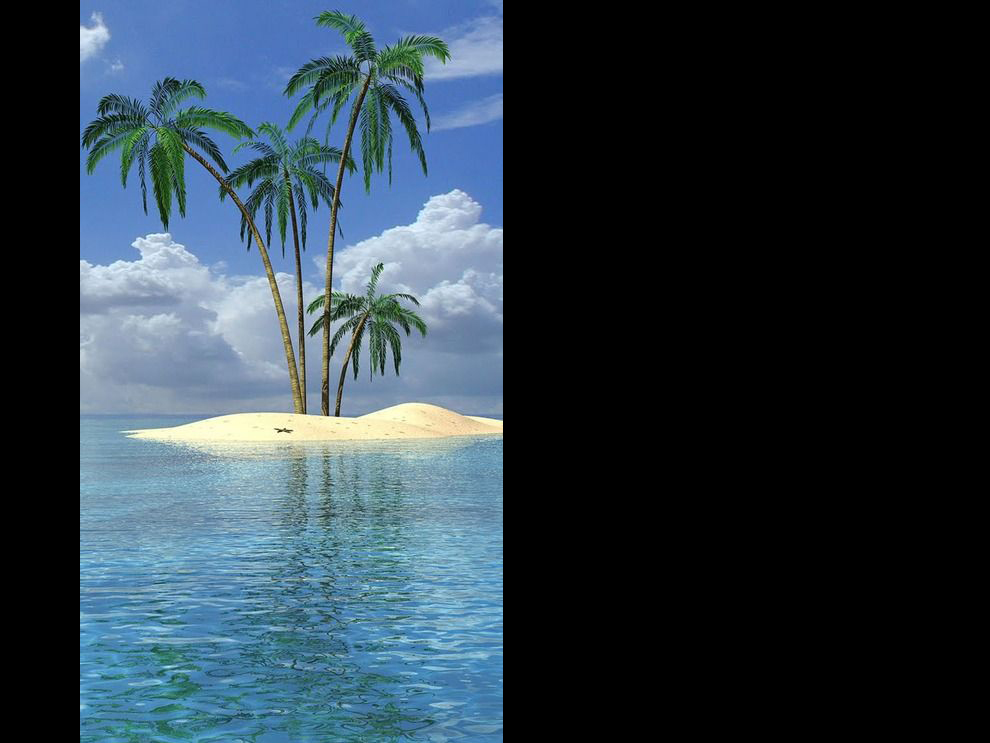 Island Source Image
|
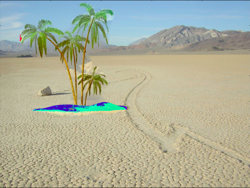 Poisson Blend
|
There were a couple of issues that made the poisson blending of the desert and the island a little difficult. One was that the source image has a very irregular shape, so a naive mask that just surrounds the overall island didn't work very well since it captured clouds in between the trees that transferred onto the sand on the desert. Another was that some areas of the source image were overly dark or overly bright, causing some irregular coloration.
Poisson Blending vs Laplacian Blending
|
Hand Original
|
Eye Original
|
Mask for eye
|
 Source pixels copied over
|
Laplacian Pyramid Blend
|
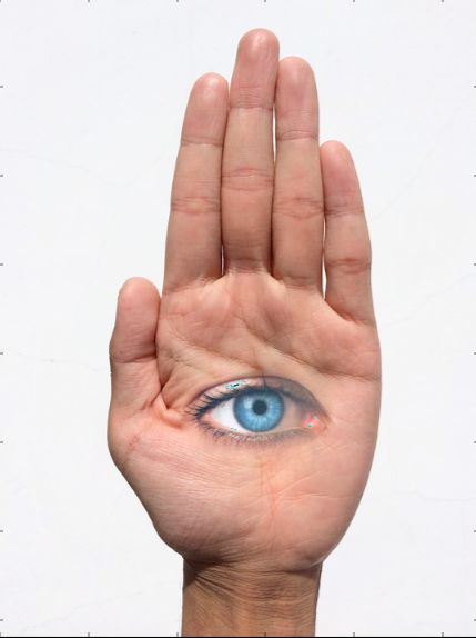 Poisson Blend
|
Here, we have 3 different blending techniques used on the Hand-Eye example from part 1.4. The Laplacian blend was done in grayscale, but it still provides a good comparison. While the Laplacian blend did blend the two images together without a noticeable seam, there are still some differences between the skin color on the hand and on the eye, as well as some textural differences. Meanwhile, the Poisson blend did a much better job in matching the skin color and textural differences between the eye and the hand (albeit there's some bright blue pixels where the highlight on the eye picture is). This shows that when it comes to overall blending of colors and textures, the Poisson works better than the Laplacian. However, if we were just trying to preserve more of the textures of the source, and just blending the seams of the two images, the Laplacian seems to do a better job of that.
Important Things Learned
The most important thing I learned from this project are the mathematical theories behind each blending technique, as well as some of the general assumptions about image perception that we leverage to develop these blending techniques.