CS 194-26 Project 3
Fun with Frequencies and Gradients!
Regina Xu (aat)
Part 1.1: Image sharpening
Overview
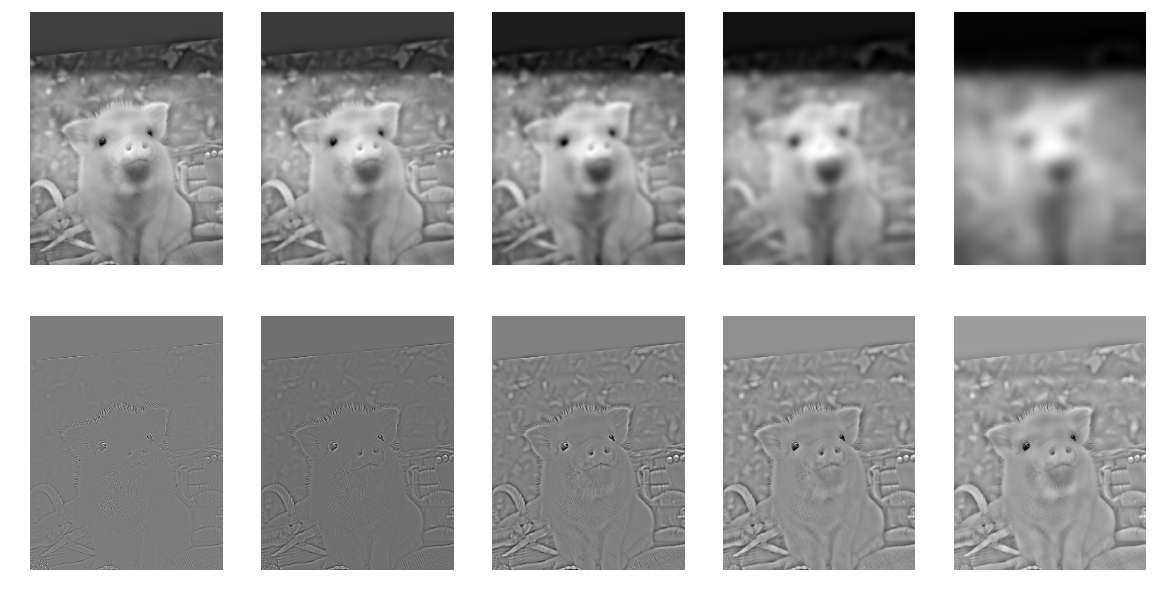
The idea is to apply an unsharp mask filter to sharpen an image, which is done by blurring an image (whose array values are divided by 255.) with a Gaussian filter then taking the difference between original image and blurred image to get the high frequency. Lastly, calculate the sum of the original and high frequency images to get a sharpened image where edges are enhanced. The equation is: sharpened = original + α*(original - blurred) where blurred is Gaussian(original).
Sharpened image with σ= 3 and α = 0.3
Clockwise from top left: original, blurred, sharpened, high frequency
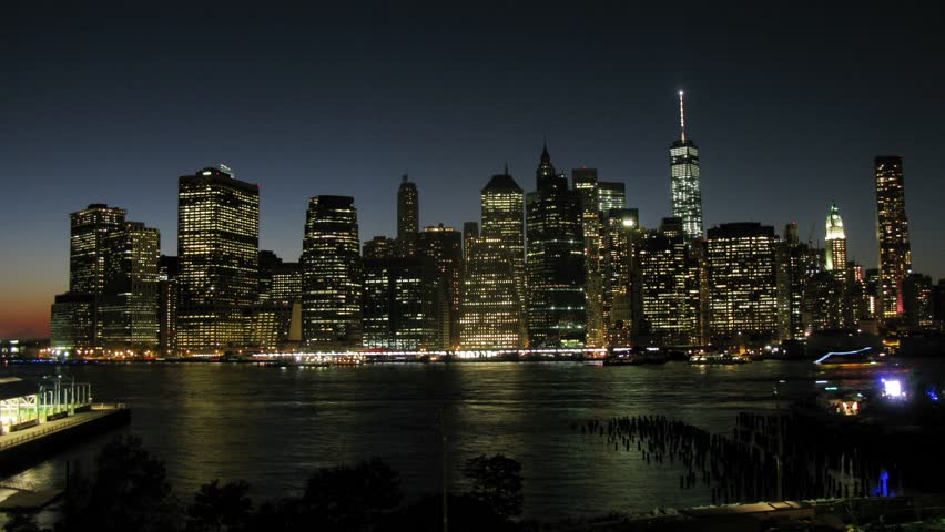
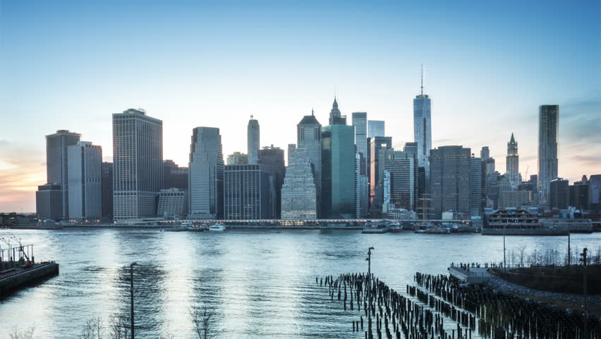
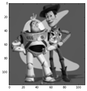
Part 1.2: Hybrid Images
Overview
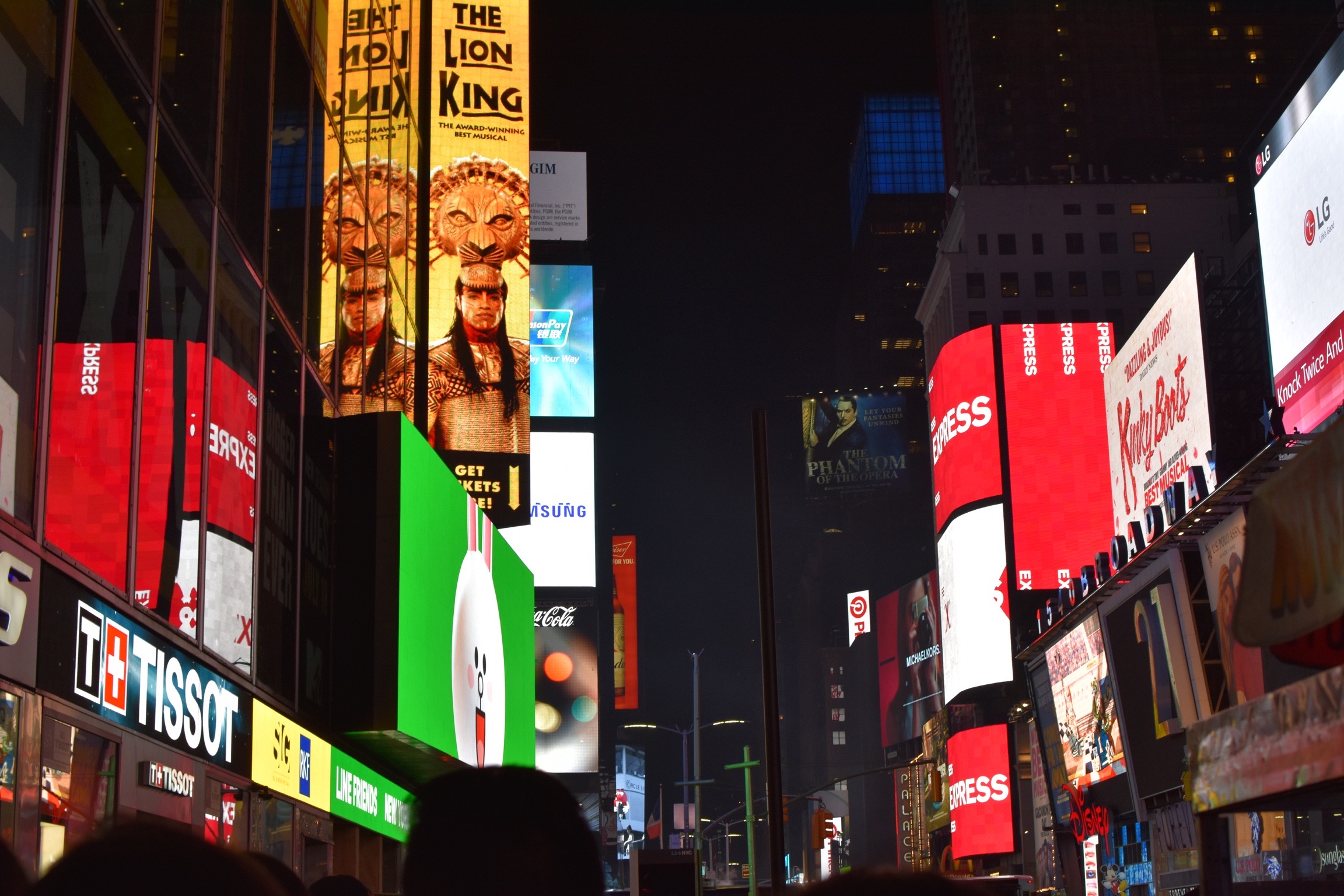
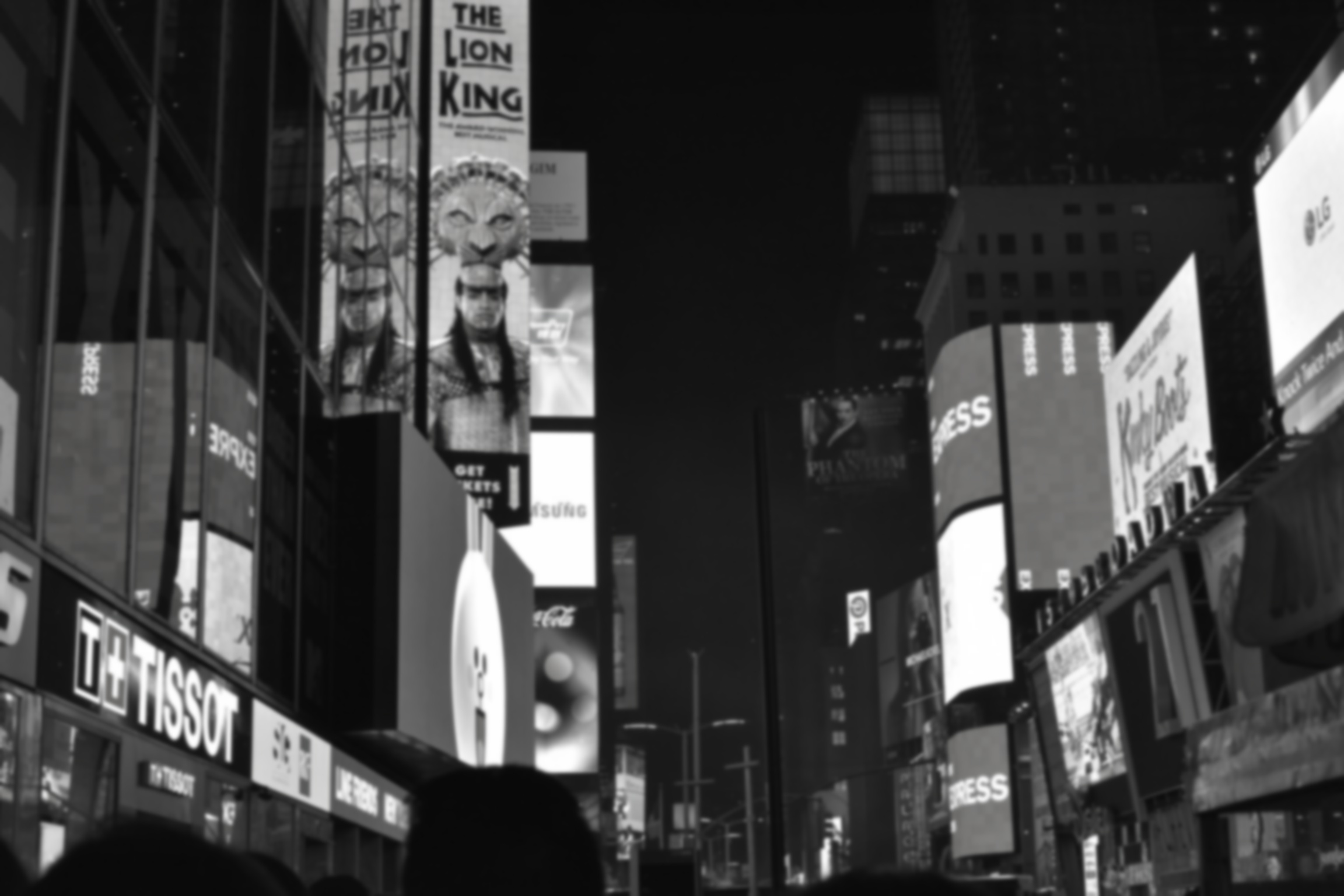
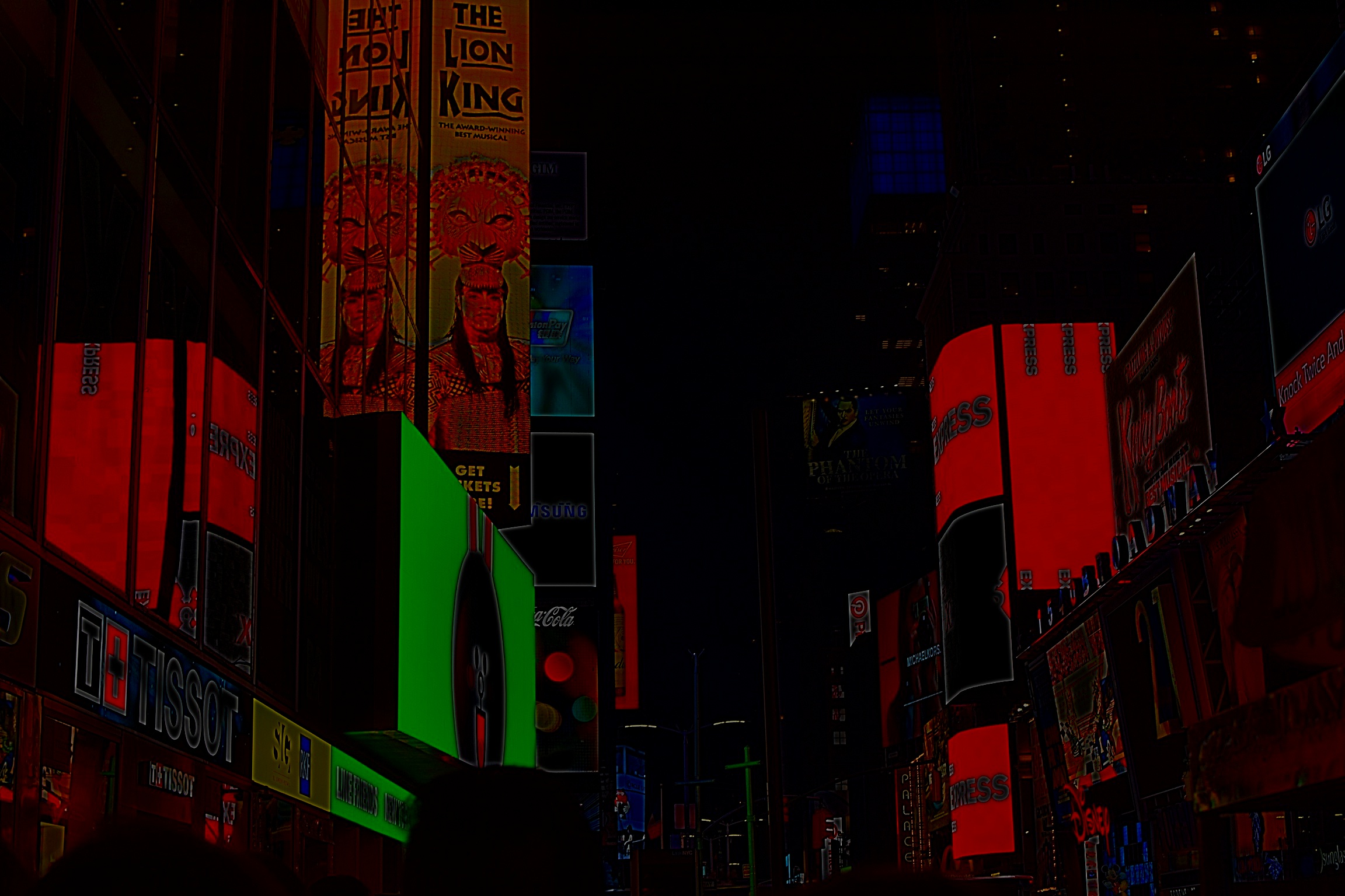
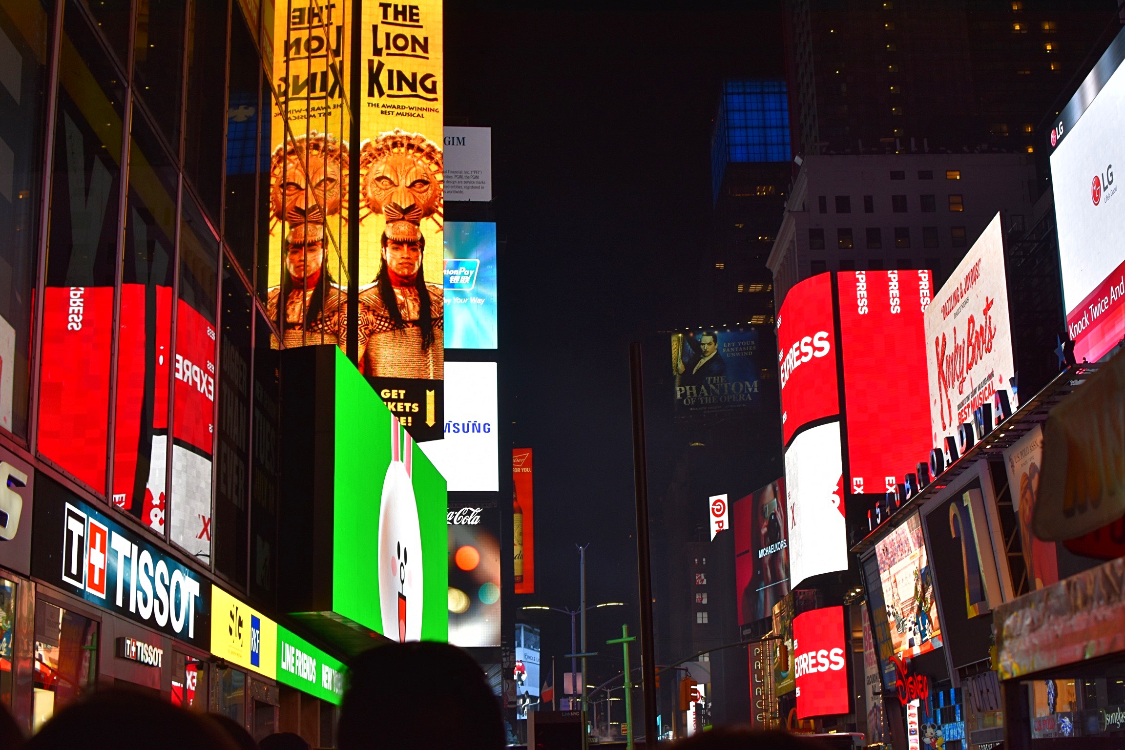
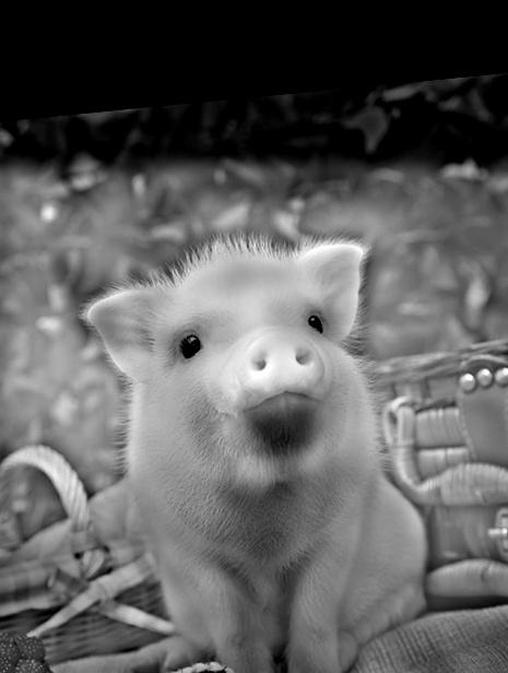
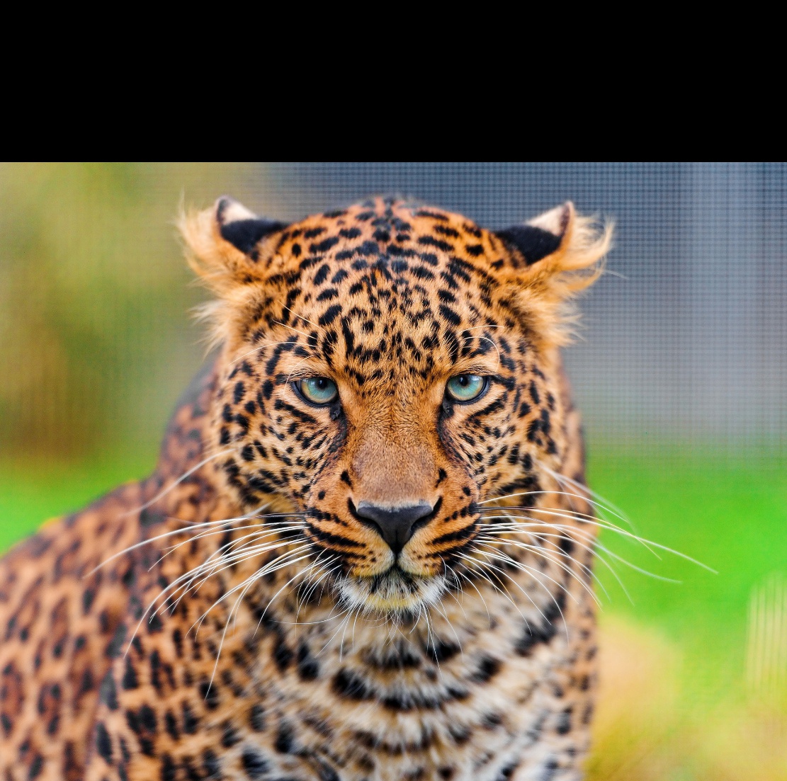
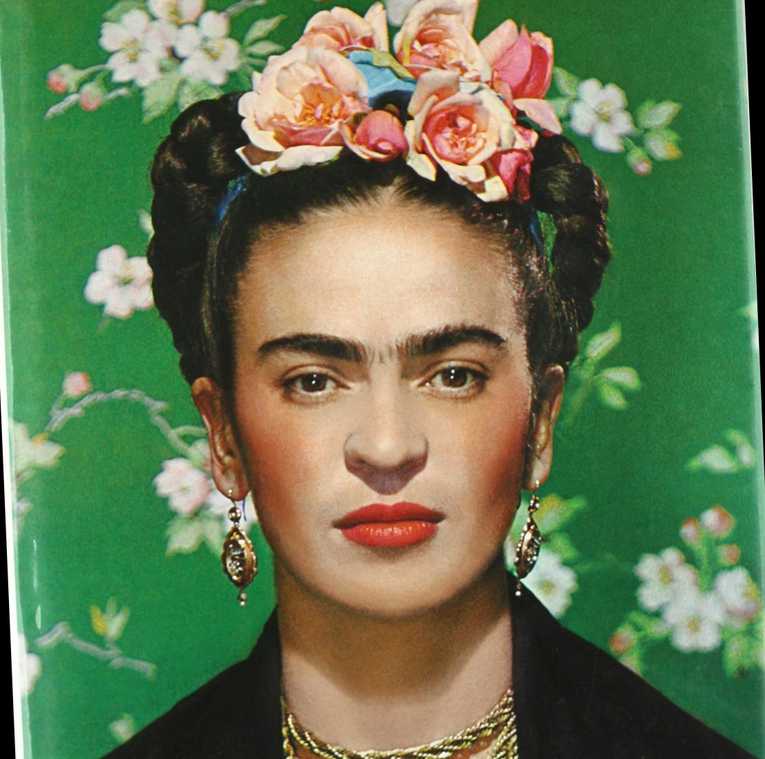
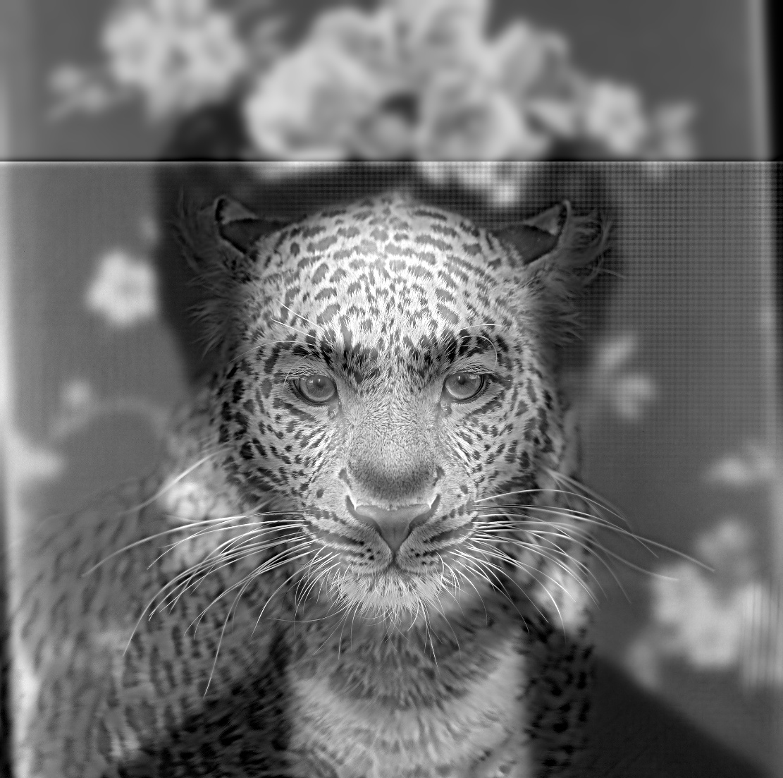
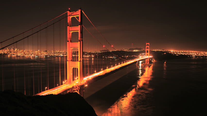
A hybrid image is created from two images at different frequencies so that at a close distance, the viewer sees the high frequency image and at a far distance, the viewer sees the low frequency image. First I run align_image_code.py with the 2 input images to get a pair of aligned images. To create a hybrid image, I combine a high frequency image with a low frequency image. Specifically, I apply a low-pass filter (the Gaussian filter) to one image, then the high-pass filter (Laplacian filter defined as original - Gaussian image) to the other, and combine them.
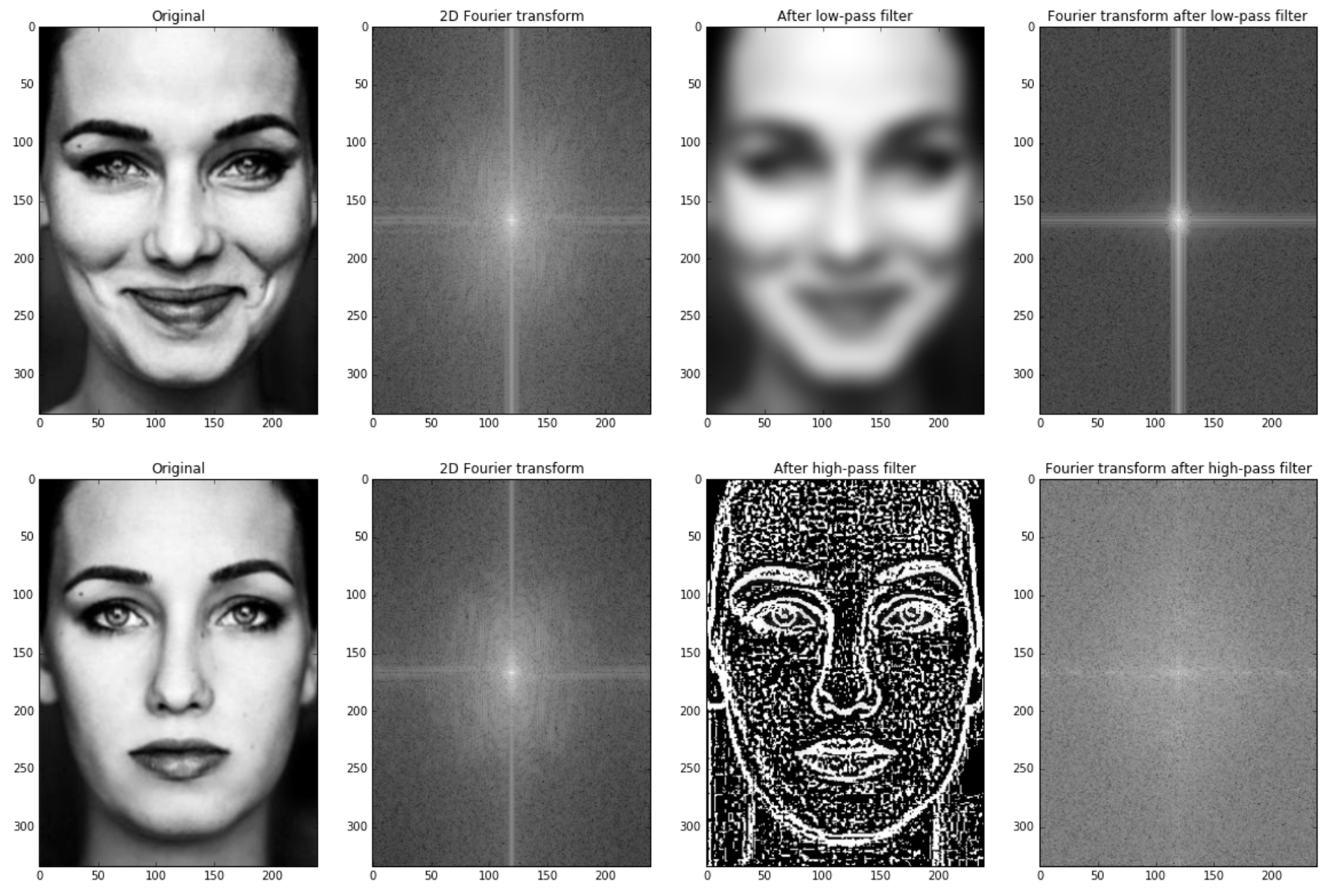
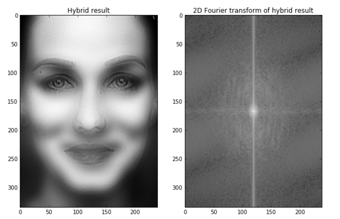
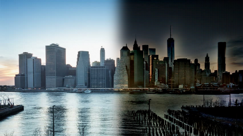
High-pass cutoff 7 and low-pass cutoff 5
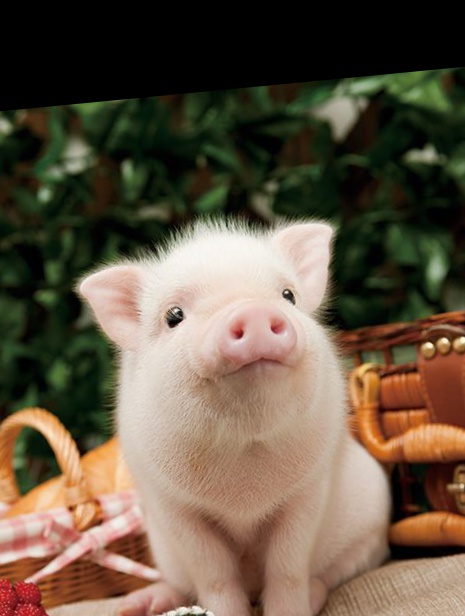
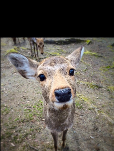
Additional results
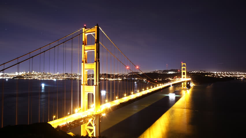
In the hybrid images below, the left image ends up as the high frequency image and the right is the low frequency image.
High-pass cutoff: 10
Low-pass cutoff: 8
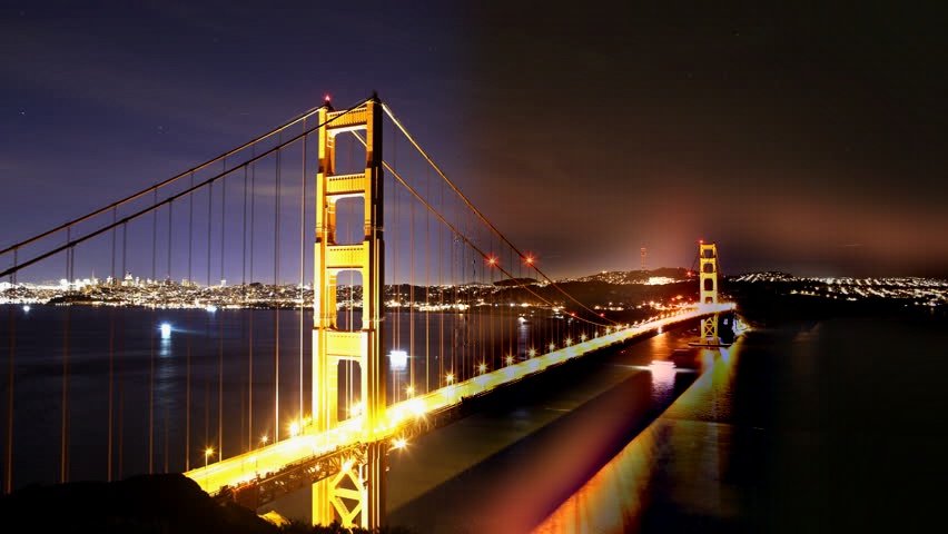
High-pass cutoff: 9
Low-pass cutoff: 5
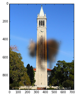
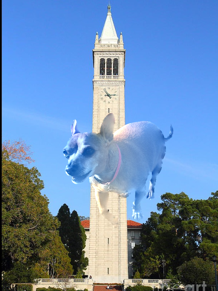
The alignment below failed due to the different widths of the input images; alignment was based on height and not width of the sharpie and Campanile.
High-pass cutoff: 3
Low-pass cutoff: 5

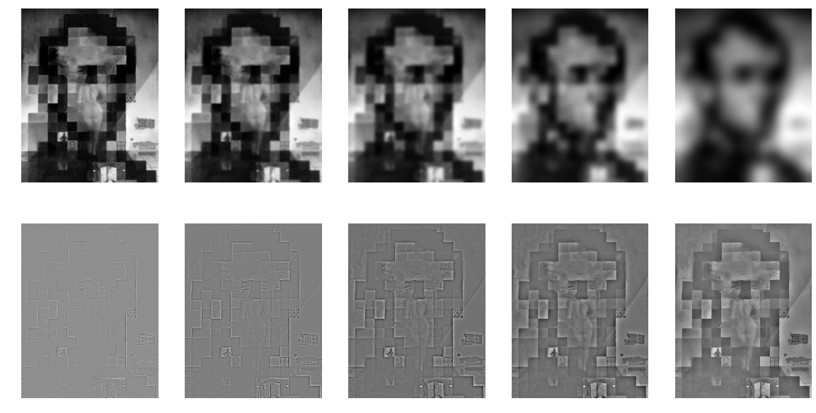
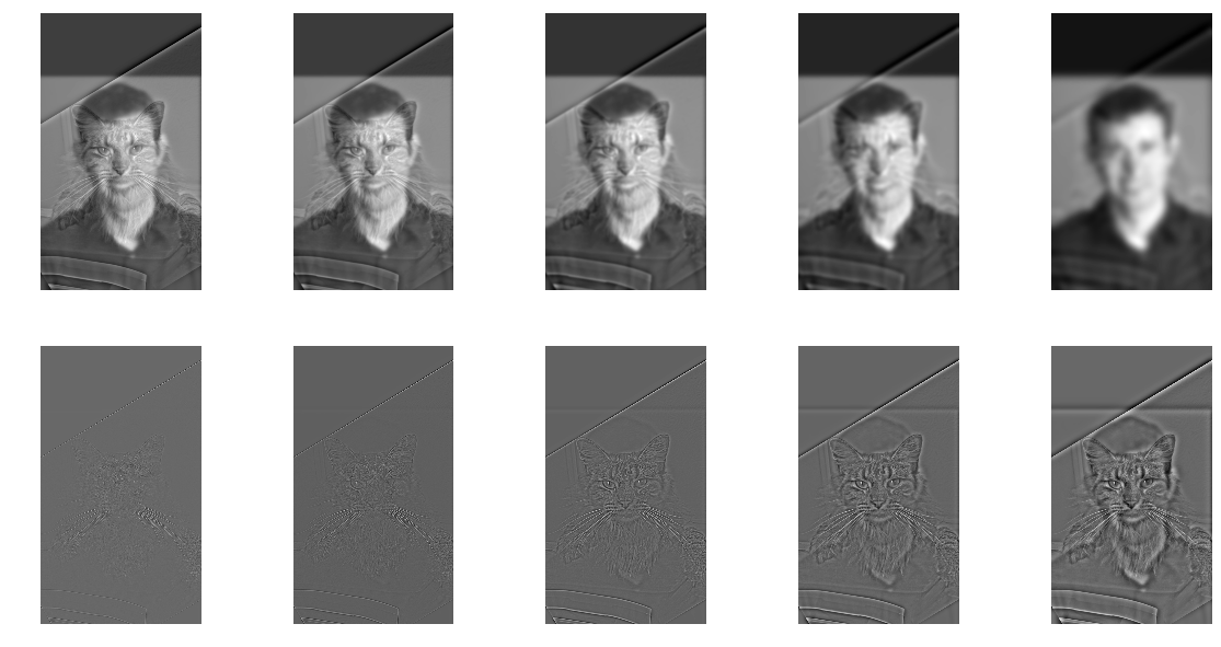
Part 1.3: Gaussian and Laplacian Stacks
The Gaussian stack applies the Gaussian filter to the input image starting with σ = 1 then σ*= 2 for each successive level. The Laplacian stack is constructed from the difference between Gaussian[i-1] and Gaussian[i].
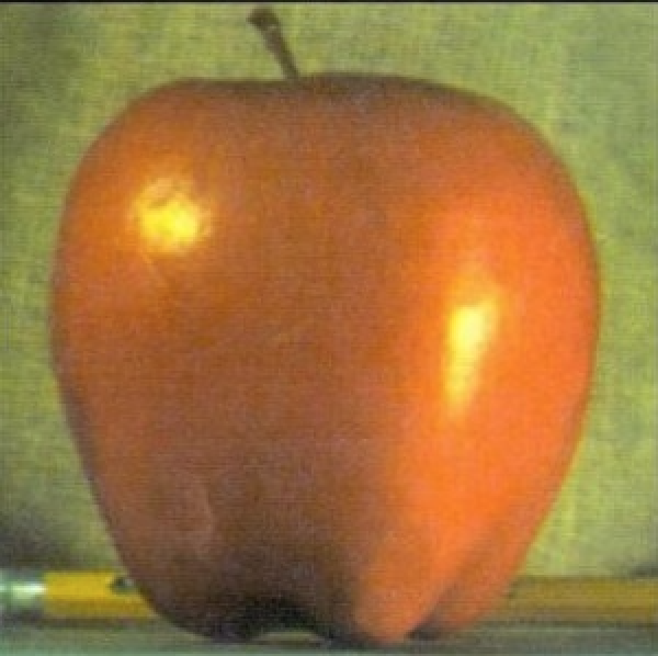
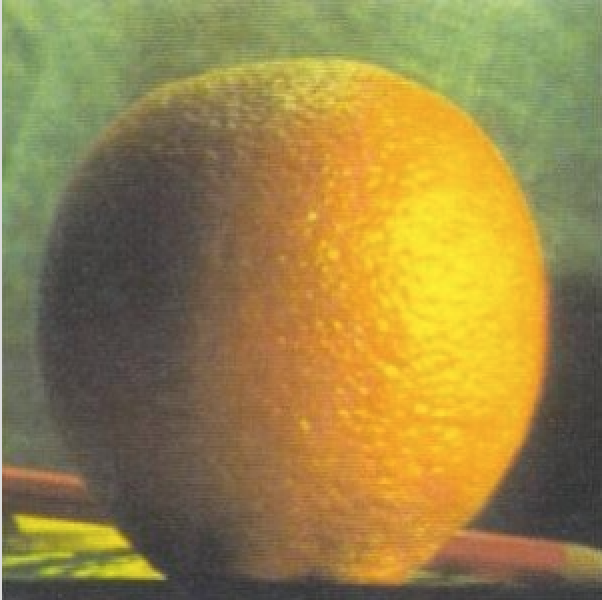
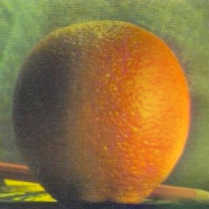
Part 1.4: Multiresolution Blending (a.k.a. the oraple!)
The idea is to combine two images into one by combining the Laplacian stacks of the images (L1 and L2) weighted by the Gaussian stack of the mask (GR), with the equation: blended = ∑i GRiL1i + (1-GRi)L2i
The input images are:
High-pass cutoff: 9
Low-pass cutoff: 5

Mask
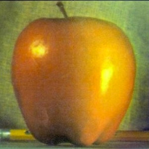
Results:
Blend of apple and orange
Additional results


Part 2: Gradient Domain Fusion
In this part, the goal is to blend a source image into a target image based on gradients or difference in pixel density. This is solved as a least squares problem of pixel intensities using gradient values and intensity of the top left corners of the images.
Part 2.1 Toy Problem
Given source image s and new image v, the three objectives are to:
1. match x-gradients of v with x-gradients of s: minimize (v(x+1, y)-v(x, y) - (s(x+1,y)-s(x, y)))2
2. match y-gradients of v with y-gradients of s: minimize (v(x, y+1)-v(x, y) - (s(x, y+1)-s(x, y)))2
3. match color of top left corners of the two images: minimize (v(1,1 )-s(1, 1))2
The approach is to construct matrix A (dimensions: 2hw+1 x hw) and vector b of gradient differences (dimensions: 2hw+1 x 1), and solve for a (hw x 1) vector of solved values that is then mapped to pixel intensities to construct the (h x w) image.
Source image (left) and new image (right)
Part 2.2 Poisson Blending
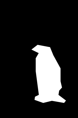
Given a source region S (image cut-out) and target region t, the goal is to seamlessly blend the boundaries of the source image region with the location in the target image. The problem is then to set v to the same gradients as the background image, aka minimize the difference between the x and y gradients. This is written as a summation over i and its 4 neighbors j (from lecture slides):

The summations are over e/ pixel i in S with j as the 4 neighbors, with the left summation matching border of S and background image. Since we don't modify t outside of S, the right summation sets v_j = t_j for j not in S (intensity value of target image).
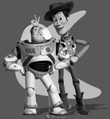
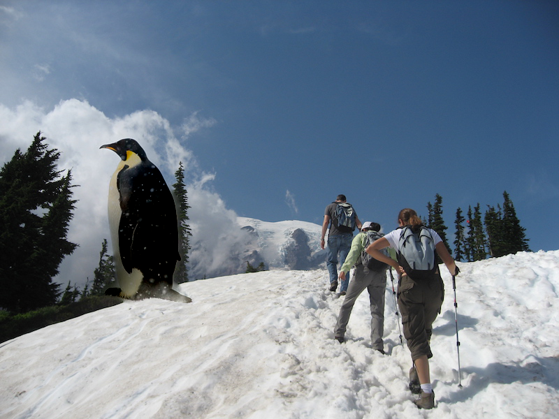
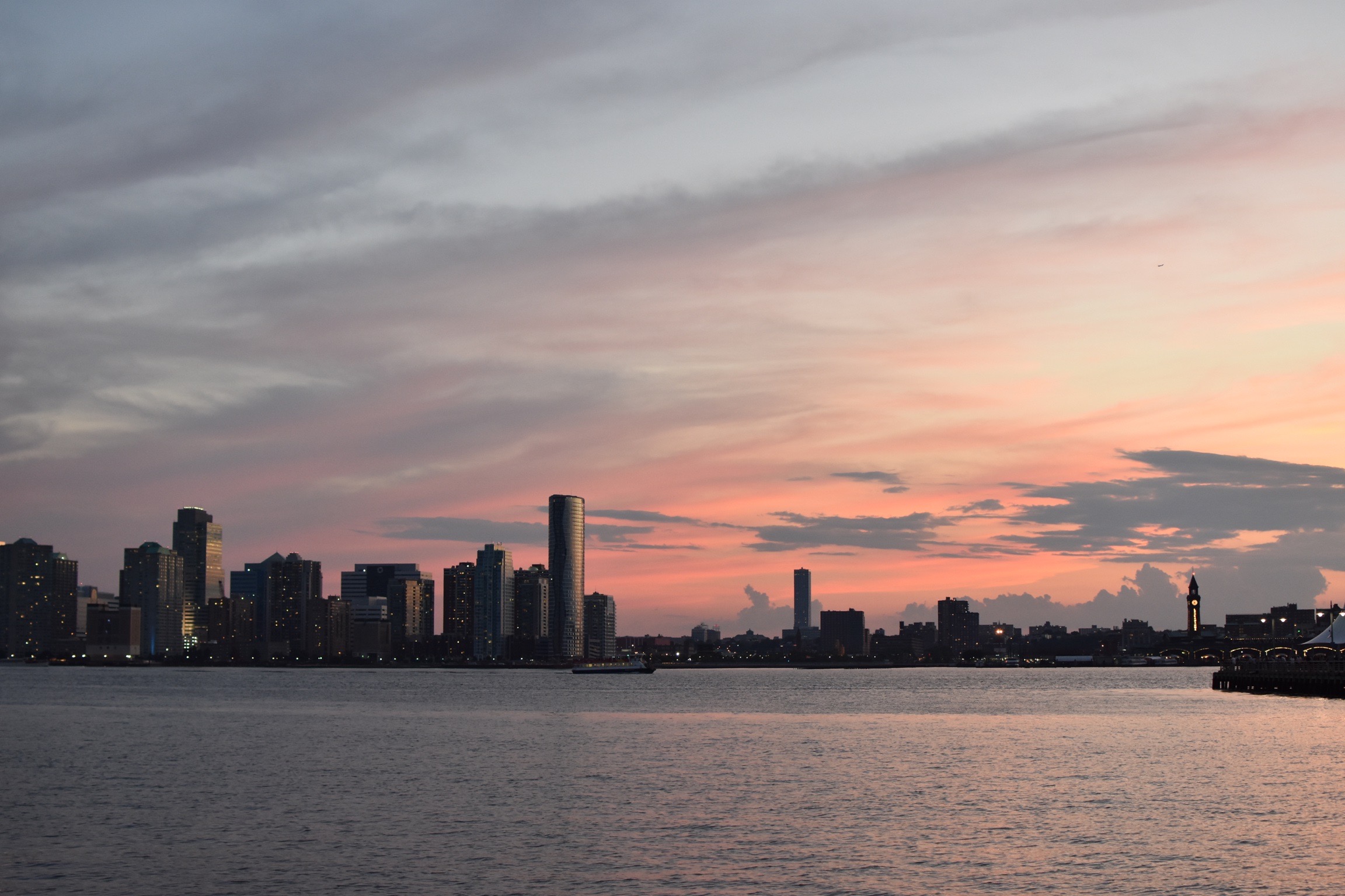
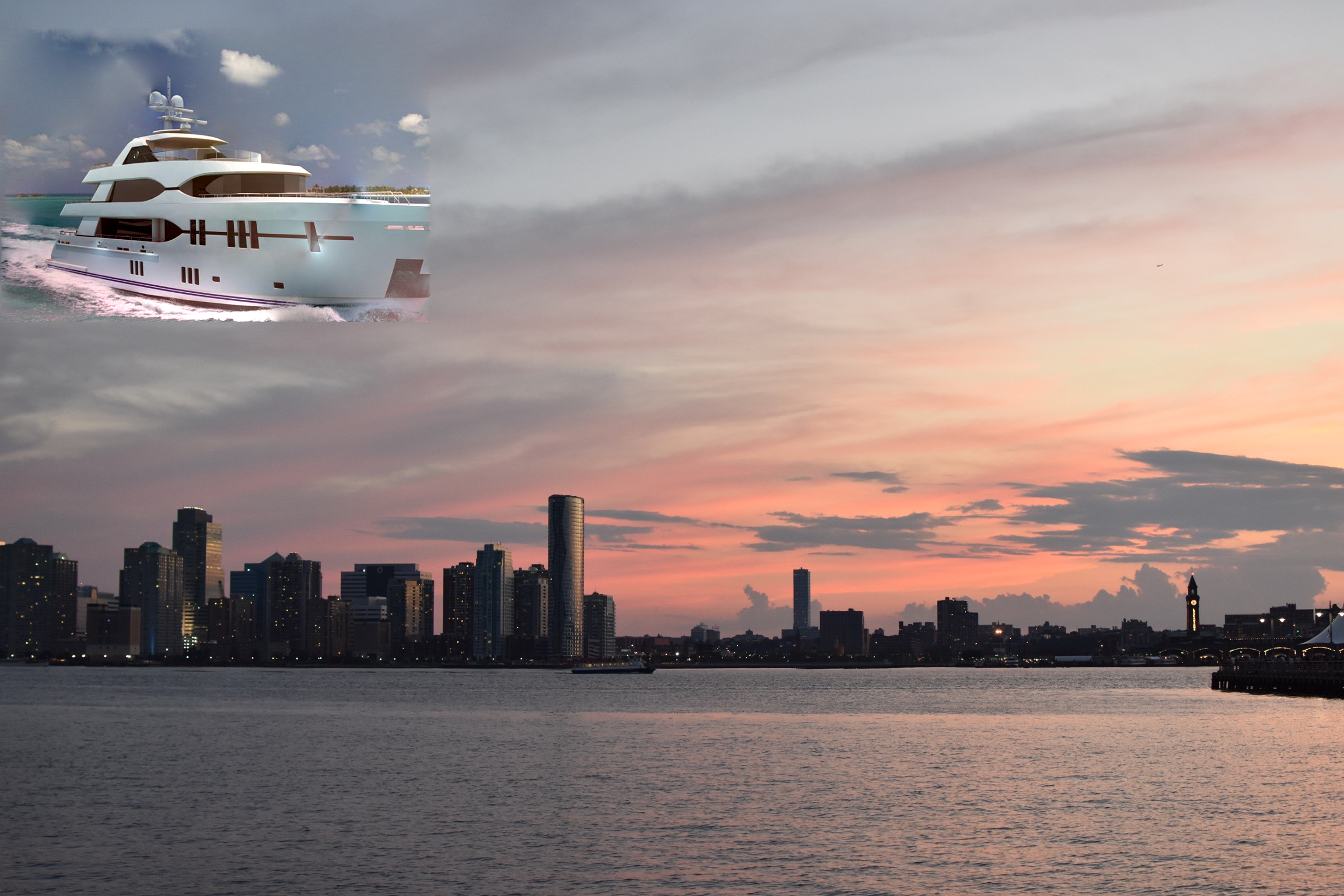
Input images: source, target, and mask
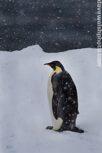
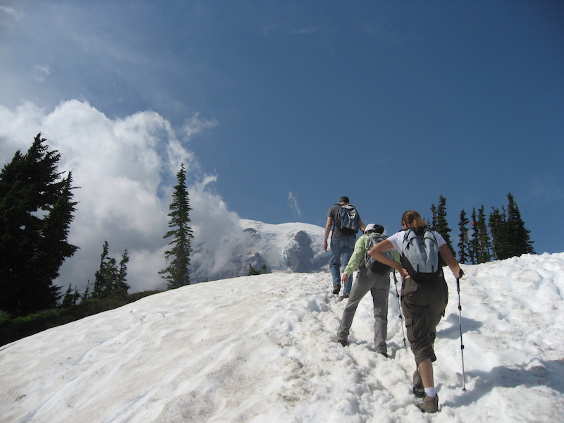
Result: since both images have snowy background, the edges of boundary seems better blended than the one below, which is where the white background of penguin image is less well-matched to the graffiti and buildings of the background image.
Same penguin and mask on different background:
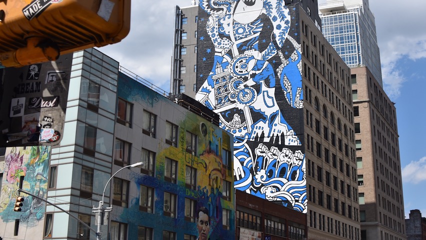
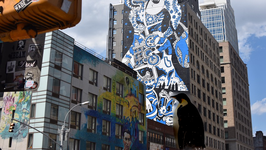
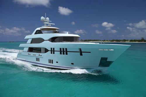
The failed image of the boat and sunset below is a result of different background colors between the source and target images.
Poisson blending vs Laplacian pyramid blending
Since my Laplacian pyramid final blending (on the left side, below) is off due to error in blending implementation, I'll make this comparison based on knowledge of the different algorithms. As seen with Poisson blending, the best output is when two input images have similar background colors, so that can also be said for Laplacian. Overall, Poisson blending is more seamless due to its underlying algorithm as a minimization of gradients versus Laplacian pyramid blending with Gaussian stack to smooth the edges of two different images.
Reflection
This project gave me a chance to get more familiar with the various library functions of SciPy and OpenCV, and through lots of trial and error, figure out the subtle parameter details, e.g. cv2.GaussianBlur vs scipy.ndimage.gaussian_filter and other differences in implementation or time complexity.