
|

|

|
|
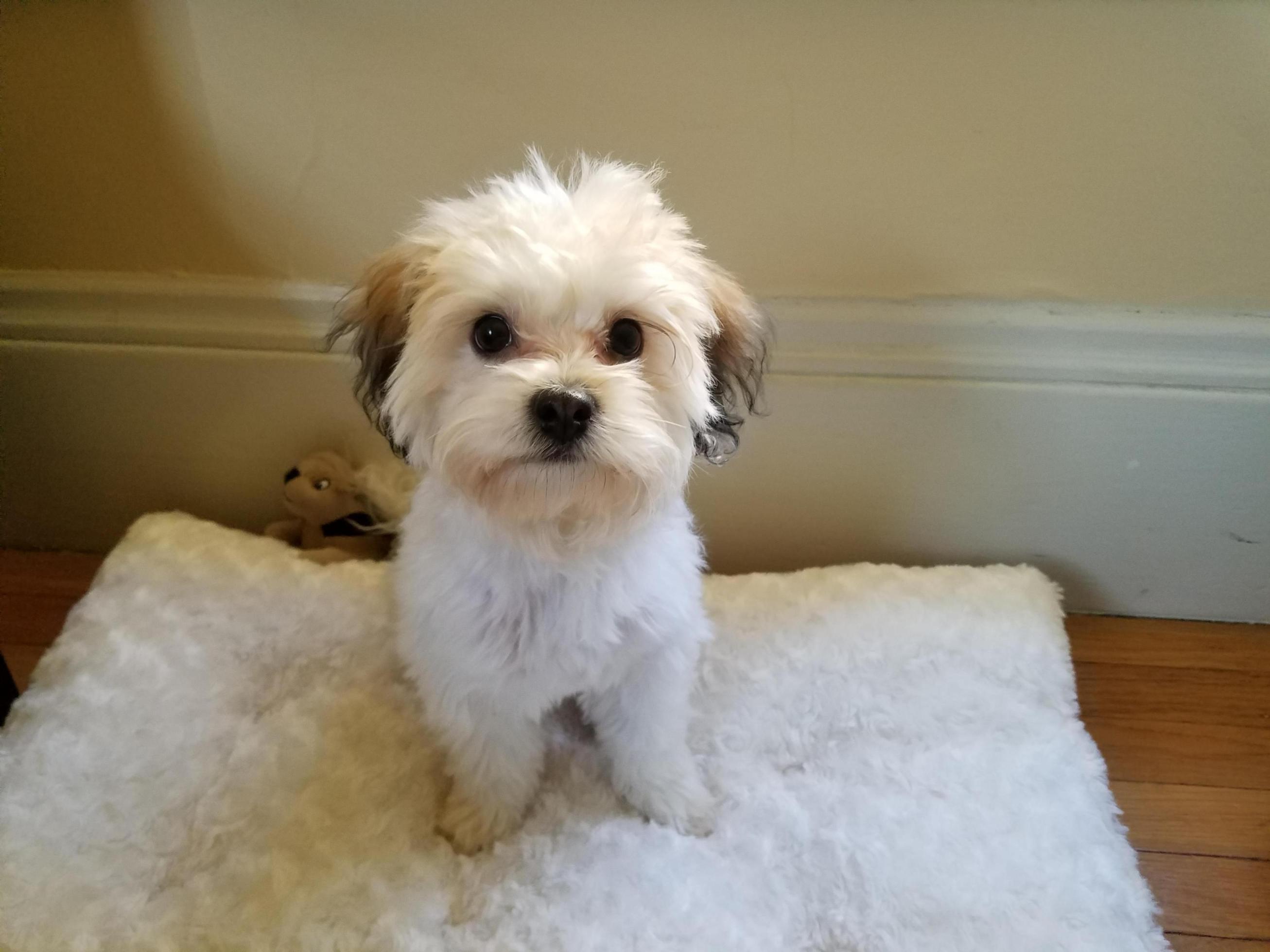
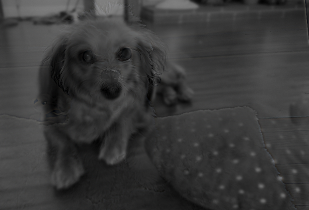
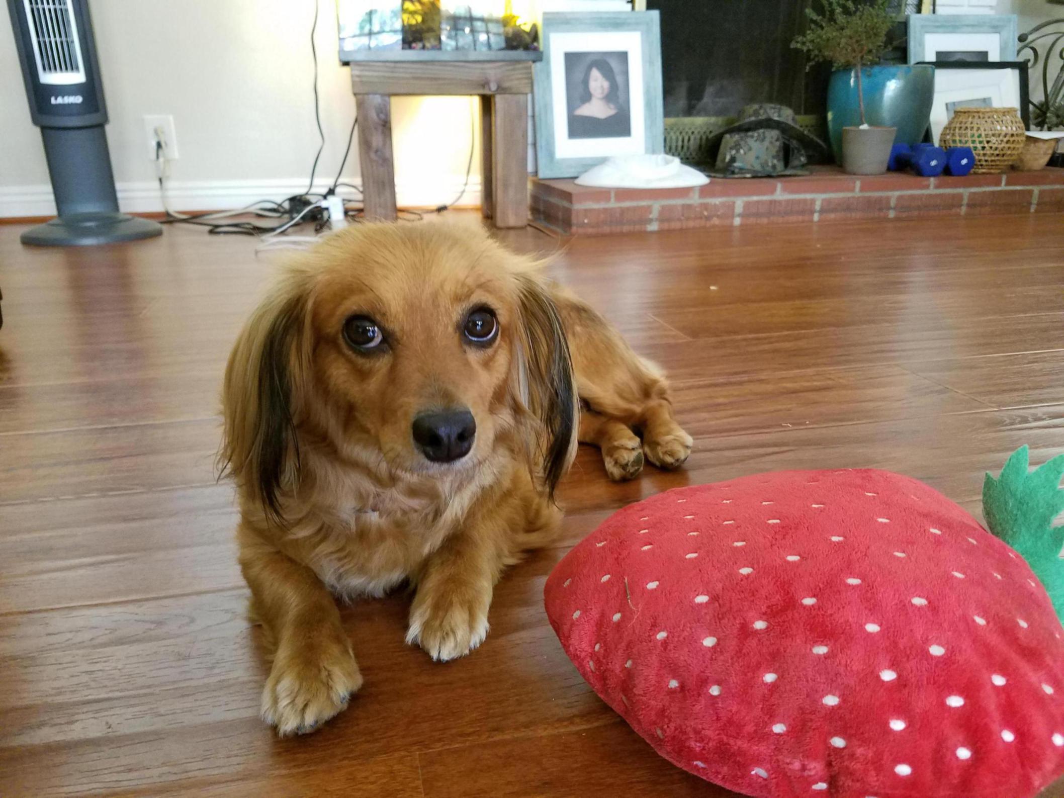
I used a slightly blurry image I found on Google and to sharpen it, I first got the low frequencies of the image using the Gaussian filter and got the high frequencies by subtracting the low frequencies from the original image.
Then I added back the high frequencies to the original image to get the sharpened image. Since it adds more signal to the original image, the sharpened images were larger in memory but looked better than the original blurry image.
However, images obtained using a very large alpha value made the image look less natural.
|
|
|
|
|
|
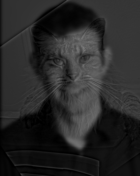
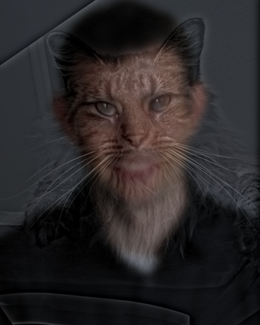
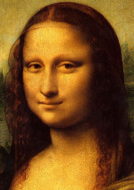
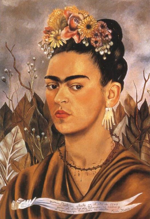
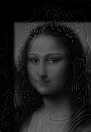
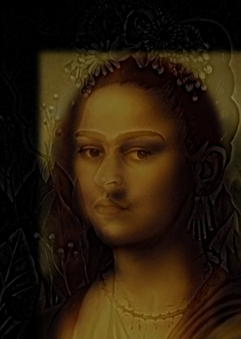
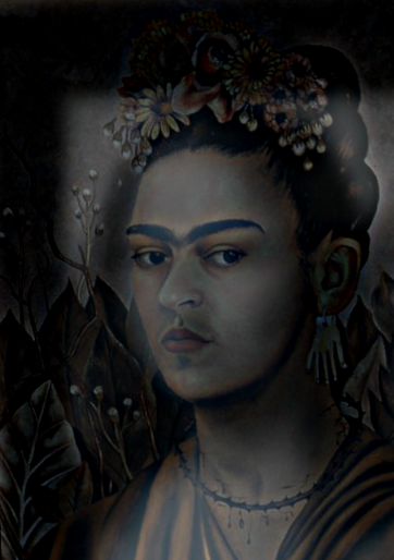
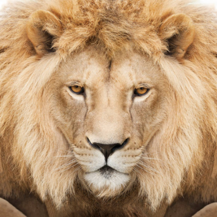
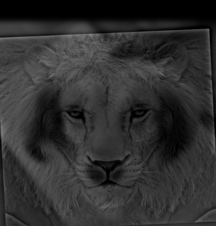
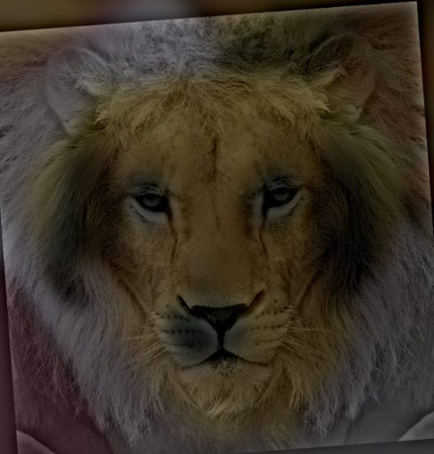
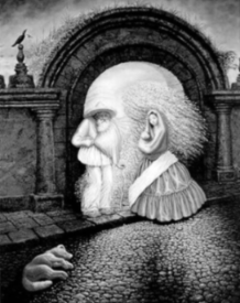
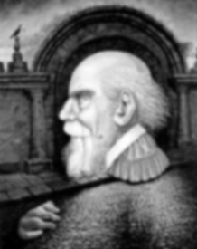
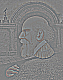
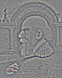
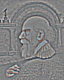
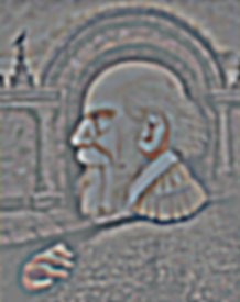
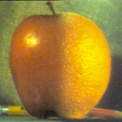
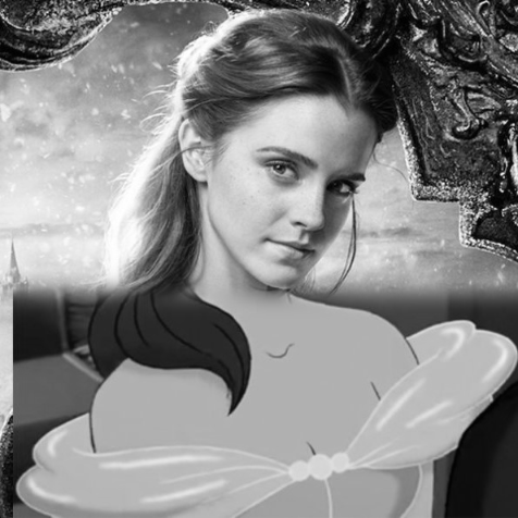
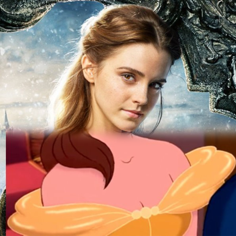
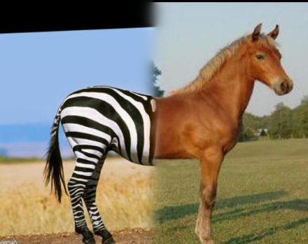
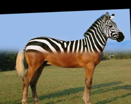
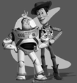
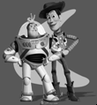
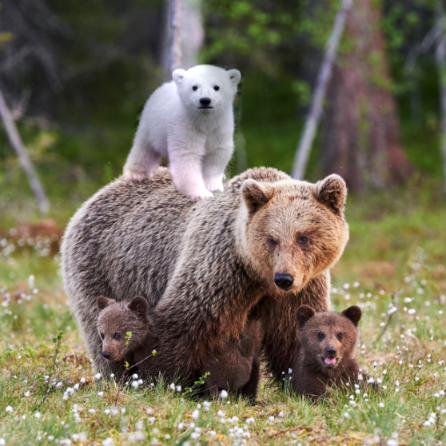
Hybrid images are images where a high frequency image is overlayed with a low frequency image, resulting in an image that looks different depending on the distance you see it from.
From a close distance, you would be able to see the high frequency image and as you moved farther and farther away, you would only be able to see the low frequency image.
To create these hybrid images, I averaged a low-pass filtered (using a Gaussian filter) image and a high-pass filtered (high = image - lowpass) image.
|
|
|
|
|
|
|
|
|
|
|
|
|
|
|
|
||
|
|
|
|
|
|
||
|
|
|
|
|
|
|
|
|
|
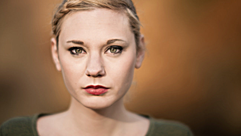
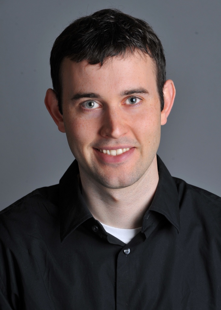
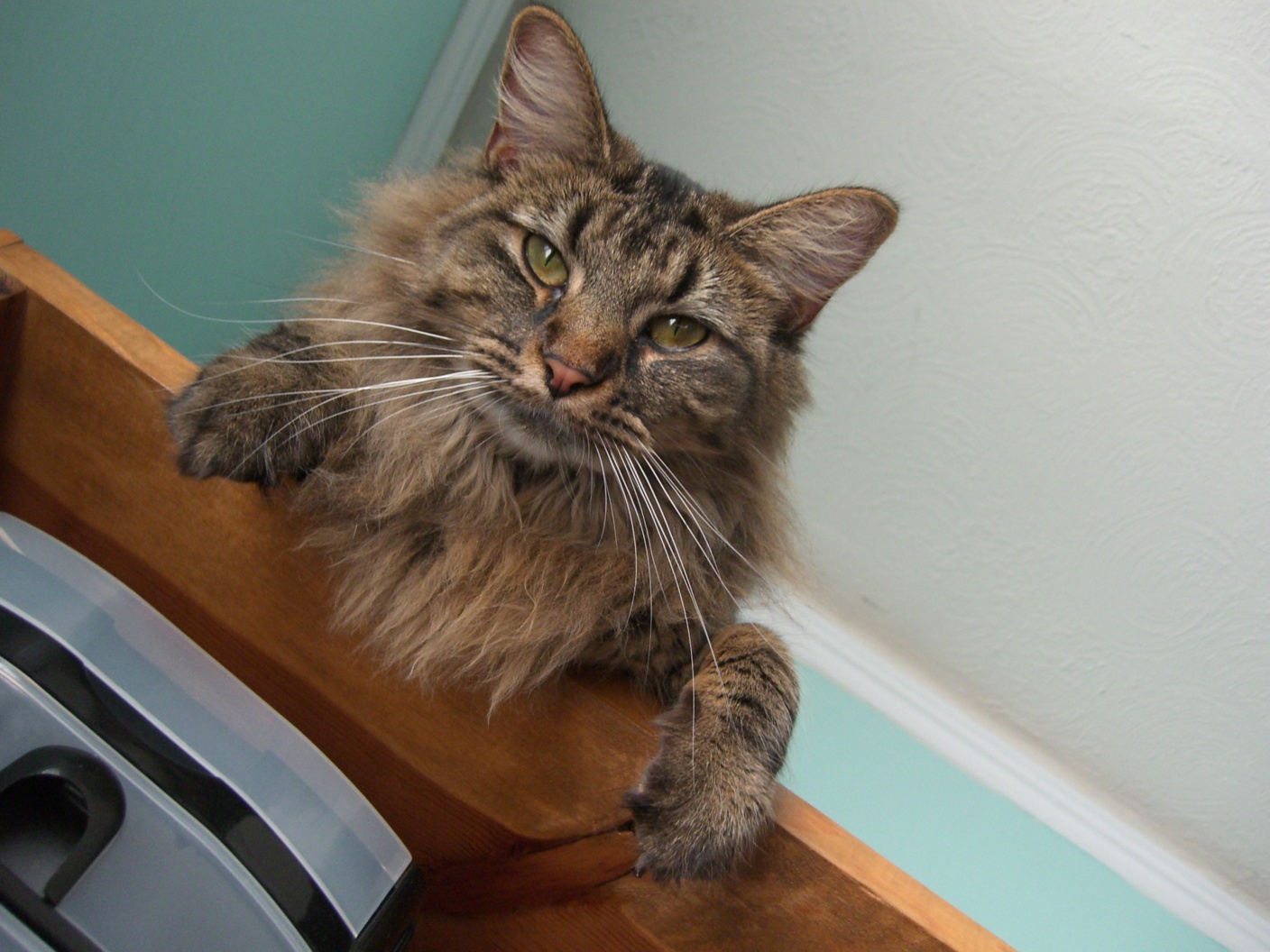
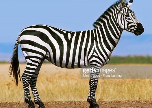
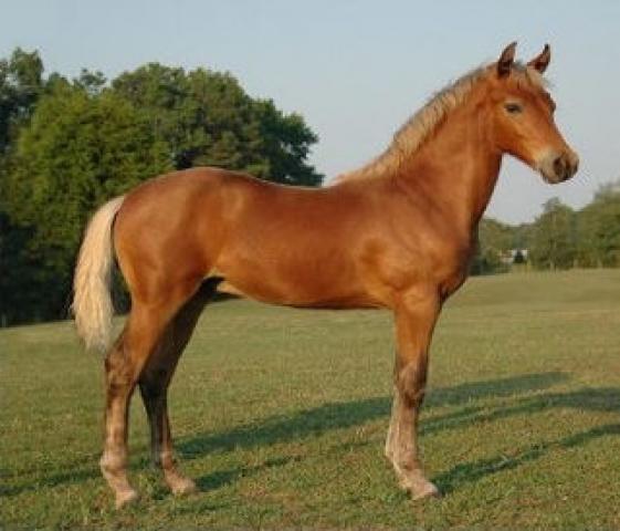
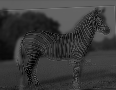
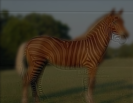
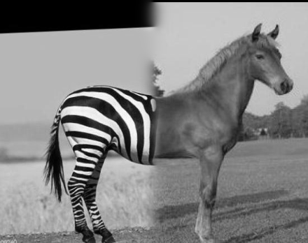
For the images I chose, I found that using color images for the low frequency images were more effective than using color for the high frequencies.
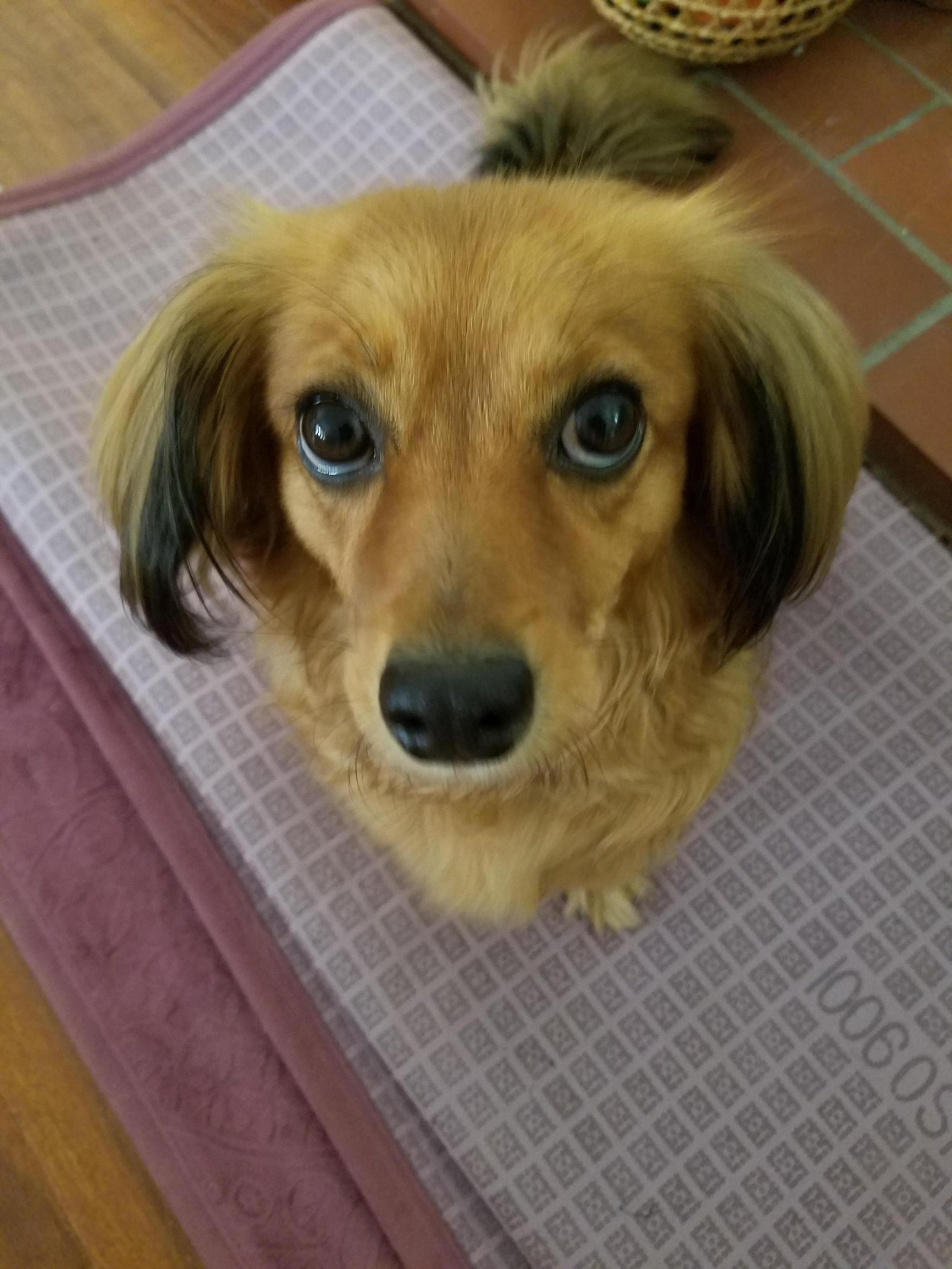
For Nutmeg, the image wasn't colorful enough to differentiate the colored image from the grayscale but using colored Derek works very well. And same for the zebra - it's already black and white so using RGB version of it wouldn't be helpful.
And for Frida and Mona Lisa, using colored Frida made the high frequency too strong so in the smaller image, you can still clearly see Frida's features. But coloring Mona Lisa works much better as you can see Frida in the larger image and Mona Lisa in the smaller.
For the fail case, it's hard to see the high frequency, probably because the grayscale images are too similar to each other.
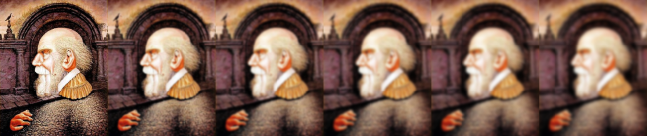
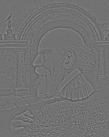
Levels of Gaussian stacks are created by applying a Gaussian filter to the original image, then on the filtered image and so on, resulting in images that become blurrier and blurrier. These images are not downsampled, which is the difference between stacks and pyramids.
Levels of Laplacian stacks are created using Gaussian stacks. To get one level of a Laplacian stack, you take an image from the Gaussian stack in the same level and an image in the lower level, and subtract them to get a high-pass filtered image of that image.
The first level in a Gaussian stack is the original image and the first in a Laplacian stack is a high pass filtered image of the original. The last image of the Laplacian will be the last image from the Gaussian stack used to create the Laplacian level before it.
Hence, in a Gaussian stack, you will be able to see the low frequencies of an image and in a Laplacian stack, you will be able to see the high frequencies of an image. Below are some examples:

|

|

|

|

|

|

|

|

|

|
|
|

|

|

|

|

|

|

|

|
|
|
|
|
|
|
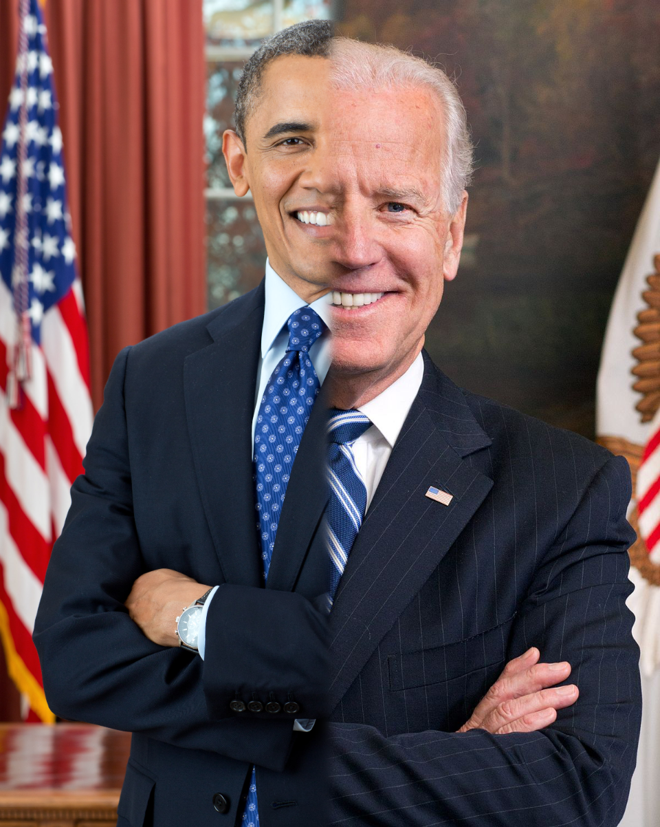
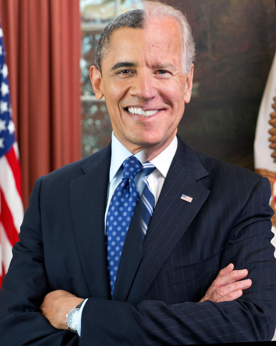
This part of the project is to blend two images seamlessly, as described in the 1983 paper by Burt and Adelson.
For this project, since we have stacks instead of pyramids, I used a mask and a Gaussian stack for the mask to blend the two images.
To create the images below, I created Laplacian stacks for both images and a Gaussian stack for the mask. Then, I used the equation from the paper
LSl(i, j) = GRl(i, j)LAl(i, j) + (1 - GRl(i, j))LBl(i, j) to combine these stacks and summed all the levels to get my results.
(Images created with uneven masks will be shown with part 2.)

|
|
|
|
|
|
|
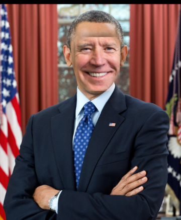
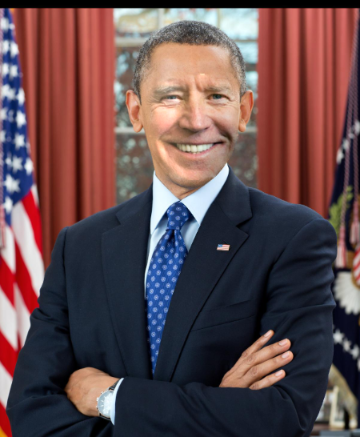
I tried blending images of Obama and Biden but without aligning them, the results weren't very good. Even with alignment, Biden's face was a little too long to match Obama's face really well.
|
|
The goal of this project is to seamlessly blend an object from a source image into a target image. The simplest way to do that would be copying the pixels from the source to the target, but it would look very unnatural unless the source and target were very similar.
So instead, we use Poisson blending, which can be formulated as a least squares problem so we can optimize and solve to get a nicely blended image.
Given pixel intensities for the source and target image, we want to solve for new intensity values within the source region for the blended image. This will preserve the gradient of the source region but overall intensity (color) may change, as shown in the images below.
To get started with Poisson blending, I started with the toy problem as a warmup. To reconstruct the given image, I used the methods described in detail on the project webpage.
|
|
The process was very similar to the toy problem, except now I had 4 * height * width constraints (for each direction/neighbor) and a target image.
Similarly to the toy problem, this problem can be formulated with least squares and optimized and solved to get the final image. I used the formulas on the project webpage to obtain my solved values, v, which I then copied into my target image. To get the final color image, I processed each channel separately and combined them at the end.
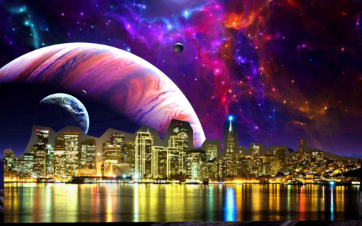
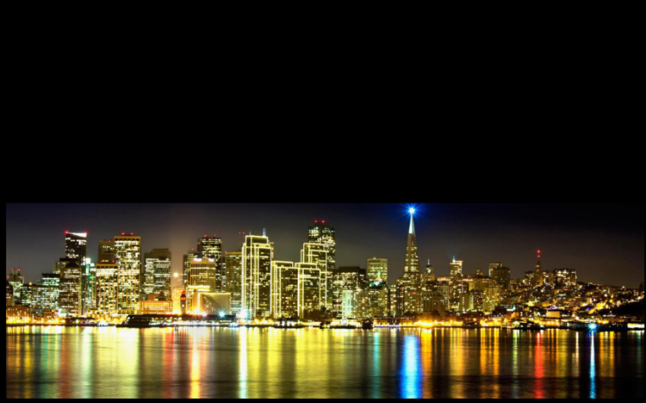
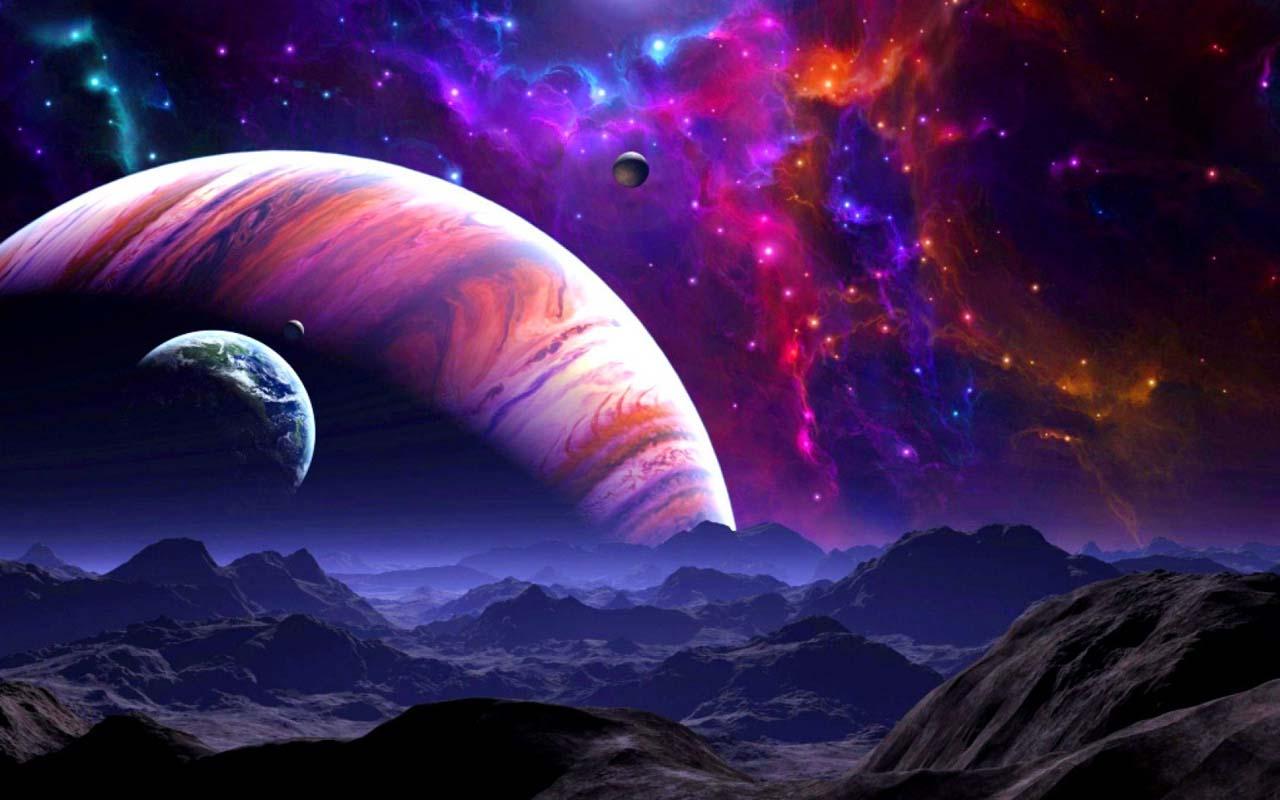
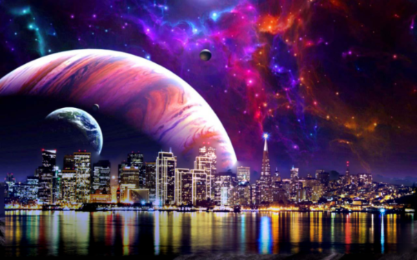
To make this process faster, I restricted my height and width to the height and width of bounding box of my mask since all other pixels would be directly copied from the target. Hence, all these images took seconds to create, except the planet and the city image, which were large images.
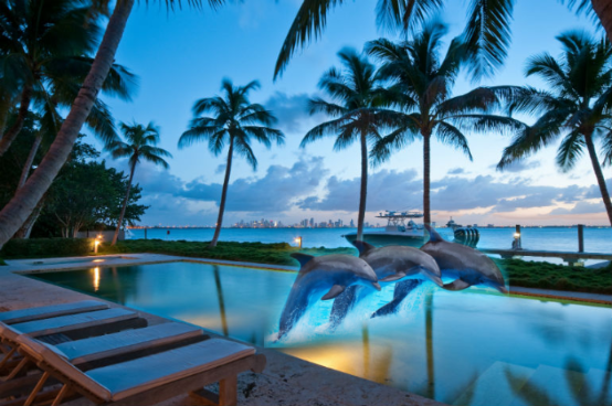
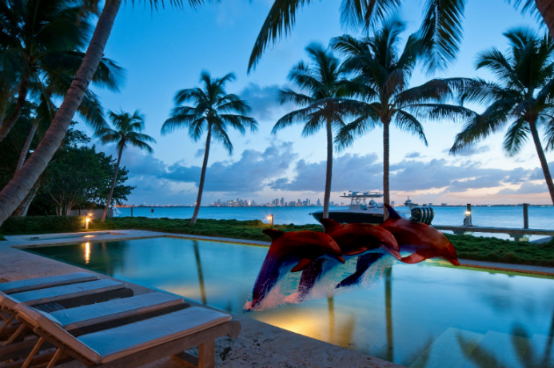
For all these images, I tried to find source images with similar backgrounds as the target images because Poisson blending would change the colors of the source image, which would make things look too unnatural (ie. dolphin, pool image).
Poisson blending works best if the source is a man-made object because the color change wouldn't make it look unrealistic (ie. green hat to red hat vs. gray dolphin to red dolphin), or if the background of the source is similar to the target because the color wouldn't change too much, making the source image look completely different.
Additionally, Poisson blending is better at seamlessly integrating the two images than Laplacian blending. Laplacian blending smooths out the edges of the source image but nothing more, so using a source image with similar backgrounds as the target would work best. And with Poisson blending, the backgrounds of source images are barely noticeable, while with Laplacian blending, you can still see the slight blur.
|
||
|
|
|

|
|
|
|
|
|
This is the only image where Laplacian blending worked better than Poisson blending because the intensity change was too strong, turning the dolphins red. Although the dolphins aren't seamlessly blended with the target image in the Laplacian, the image still looks much more natural.
|
|
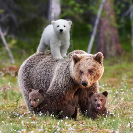
I used the same code as the code used to generate my Poisson blended images, except for the constraints. Instead of only using the source gradient, I used the gradient in source or target with the larger magnitude.
This method works best for inserting objects with holes into a target image with texture.
|
|