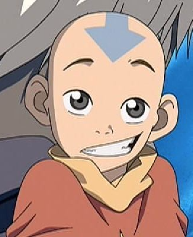
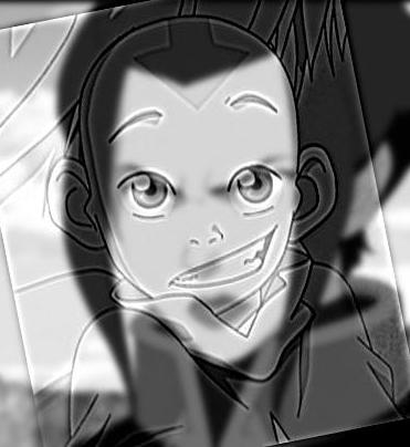
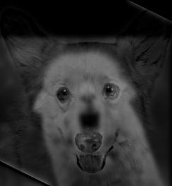
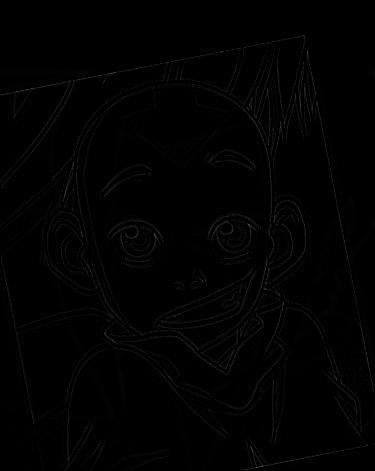
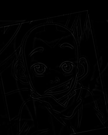
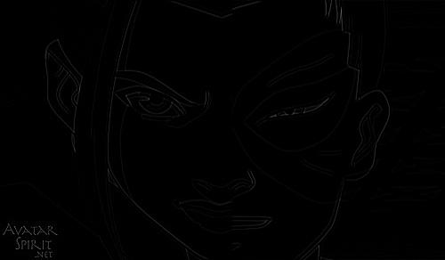
Aang
This is the image used for the high frequencies.
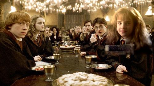
Fun with Frequencies and Gradients. In this project, we learned various techniques that dealt with the frequencies and gradients within our images.
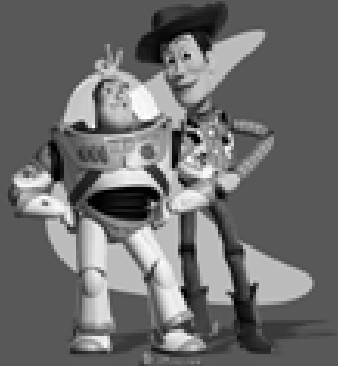
We used a Gaussian filter to blur our image, subtracted the blurred image from the original image to extract the high frequencies, and then added the high frequencies (multiplied by an alpha value) back to the original image in order to get our sharpened image. The sharpened image is on the right. I used a sigma value of 3 and an alpha value of 1.
We created hybrid images by applying a low pass filter to one image and extracting the high frequencies of the second image. .
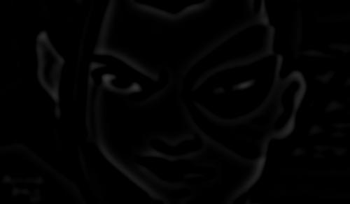
We created hybrid images by applying a low pass filter to one image and extracting the high frequencies of the second image (by subtracting the original image by the gaussian filtered image). We added the results together to produce a hybrid image. I used a sigma value of 3 for the high frequency image and a sigma value of 2 for the low frequency image. We can see that the hybrid image isn't perfect and that the images don't align too well. The two characters have very different facial structures and aren't looking in the same direction. However, from up close, Aang, as the high frequency image, dominates the vision and he is almost unnoticeable from a distance as Azula takes over. Below, we have the images used on the left and their corresponding 2D Fourier Transform. I also included other images and their hybrids, where some turned out better than the Aang/Azula image. Click on each image to view their full size. (Note: Only the FFT and actual hybrid images will have full size images - the others won't load due to the size constraint of the upload).
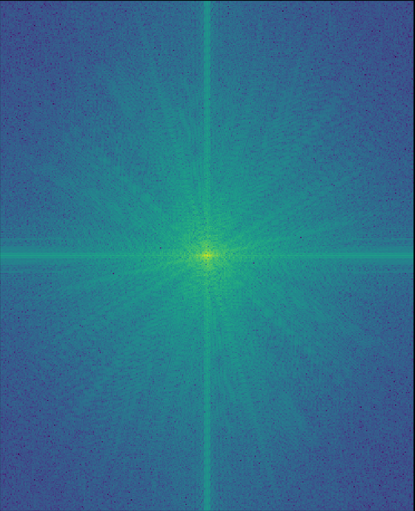
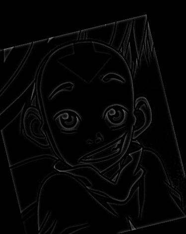
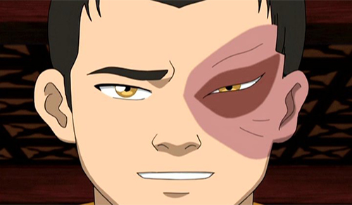
This is the image used for the high frequencies.
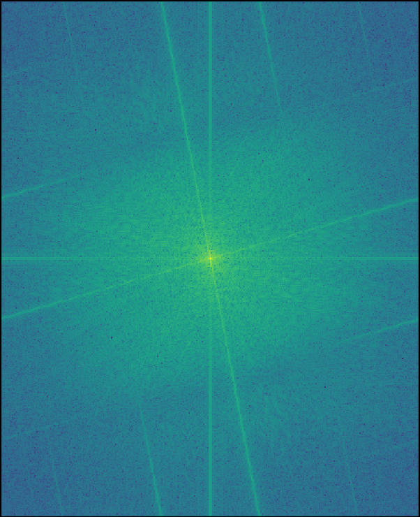
The log magnitude of the Fourier transform.
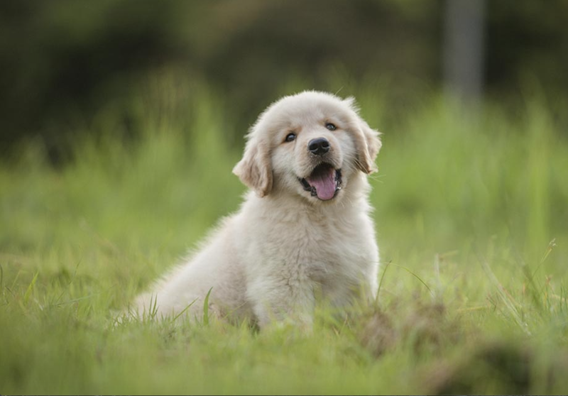
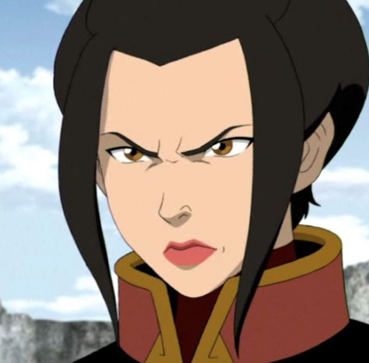
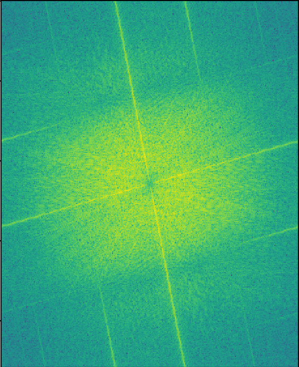
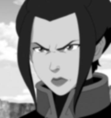
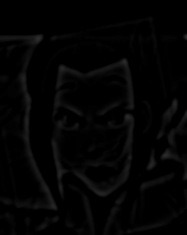
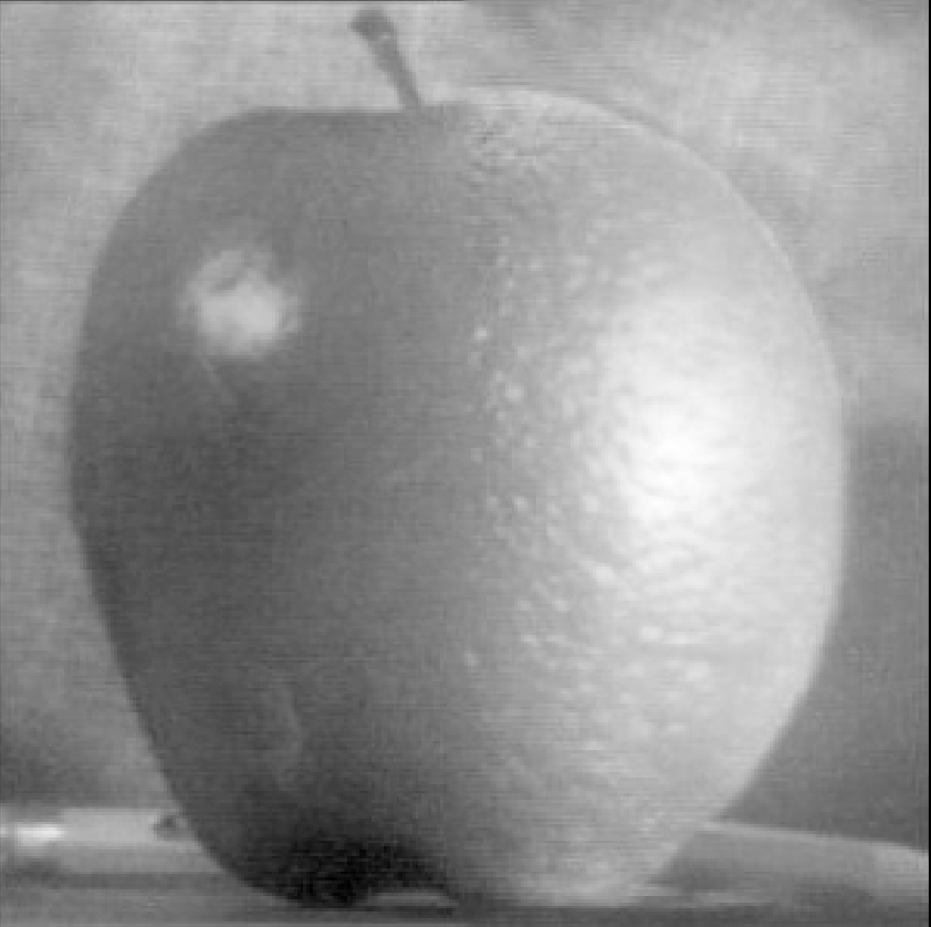
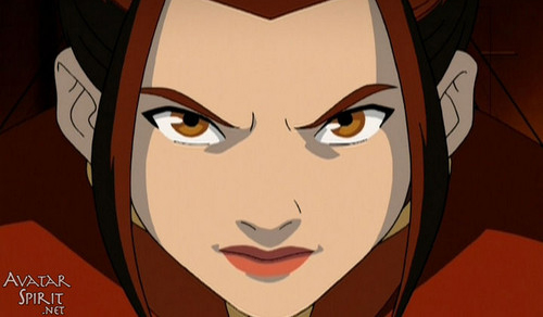
This is the image used for the low frequencies.
The log magnitude of the Fourier transform.
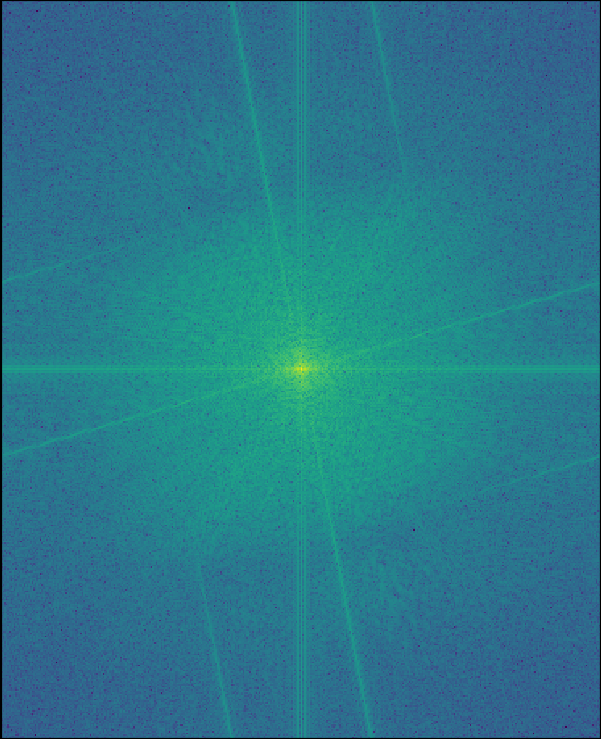
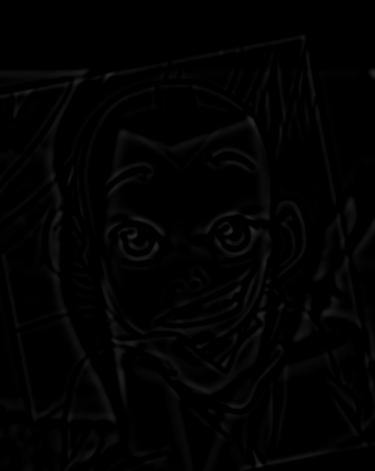
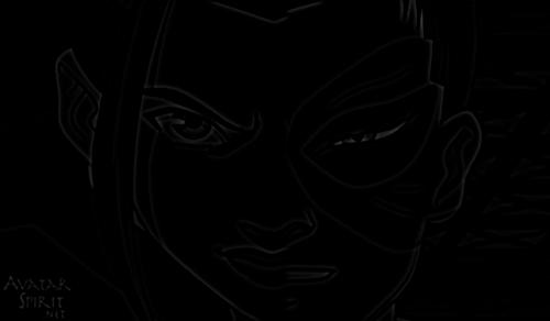
This is the Aang image with the impulse filter applied (1 - the gaussian filter on the image).
The log magnitude of the Fourier transform.
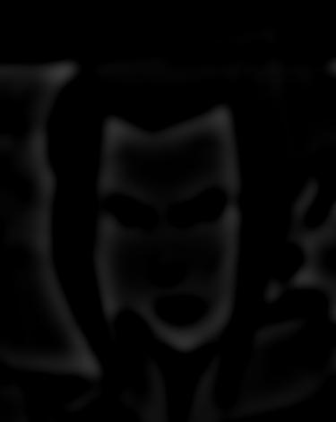
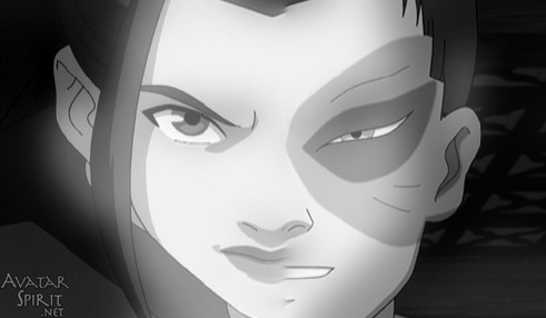
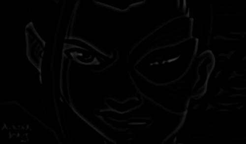
This is the Azula image with the low pass filter applied (the gaussian filter).
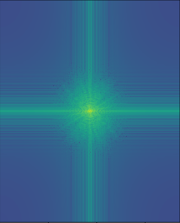
The log magnitude of the Fourier transform.
The hybrid image of Azula and Aang.
The log magnitude of the Fourier transform.
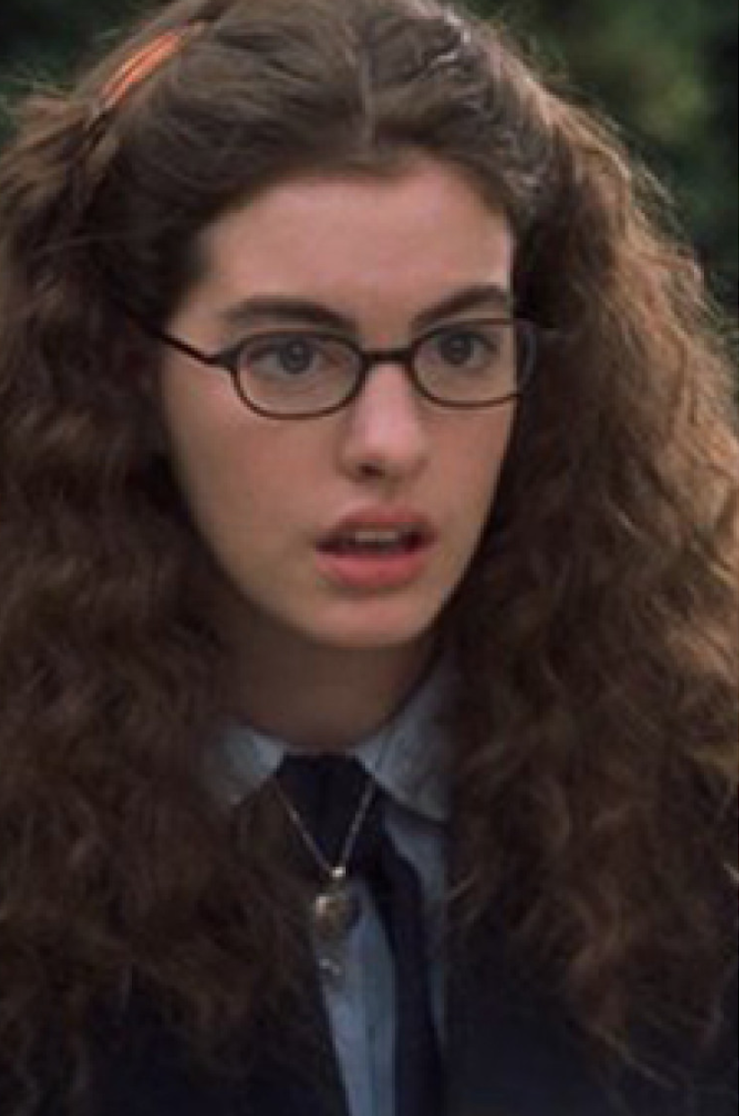
This is the image used for the high frequencies.
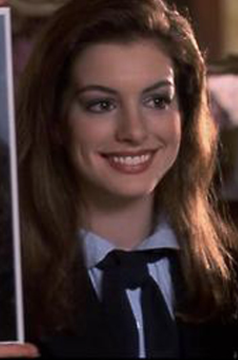
This is the image used for the low frequencies.
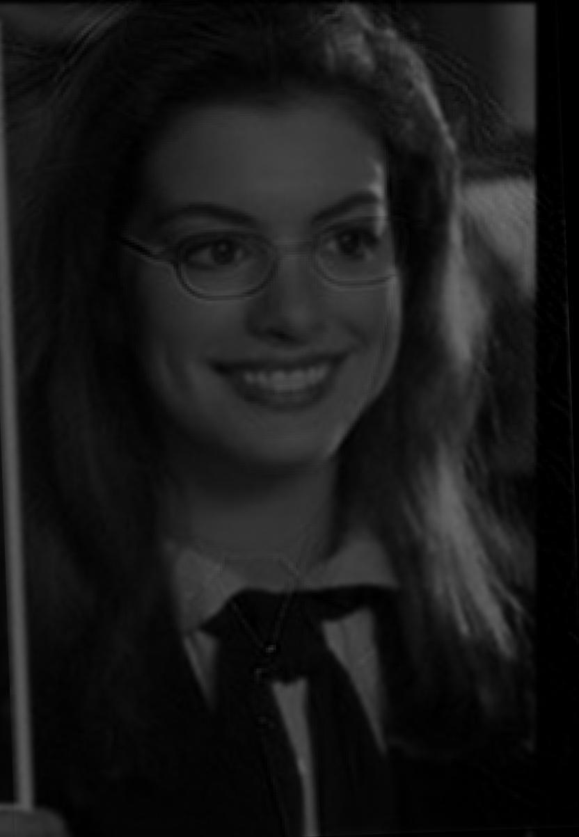
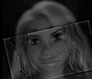
This is the hybrid image of Mia before and after her makeover.

This is the image used for the high frequencies.

This is the image used for the low frequencies.
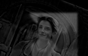
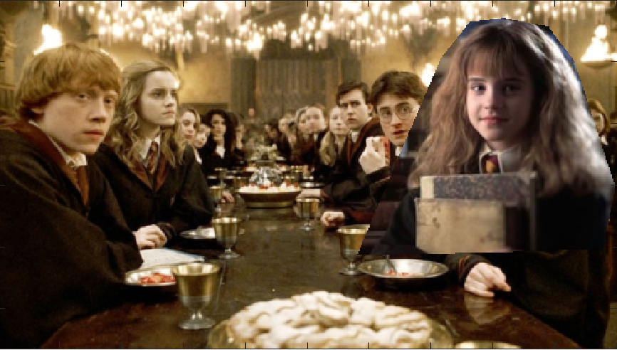
This is the hybrid image of Emma and Belle.

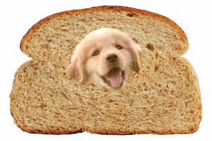
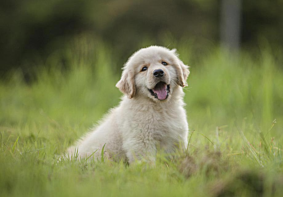
The is the image used for the high frequencies.
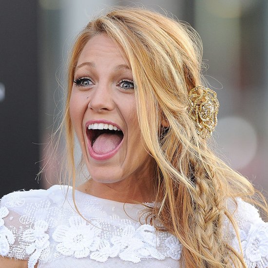
This is the image used for the low frequencies.
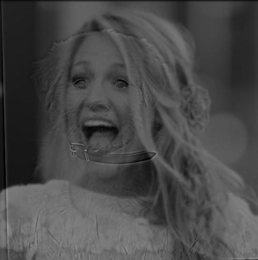
The is the hybrid image of Blake and the pupper.

The is the image for the high frequencies.

The is the image for the low frequencies.
The is the hybrid image of the corgi and the llama.

The is the image for the high frequencies.

The is the image for the low frequencies.
The is the hybrid image of Mandy Moore and Rapunzel.
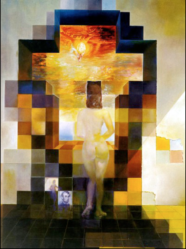
We built a Gaussian stack by applying a Gaussian filter to the original image at each layer, x, with a sigma value of 2x.


We built a Laplacian stack by taking the difference between consecutive Gaussian layers. The last image is the reconstruction of the Lincoln image after adding all the Laplacian layers together along with with the final Gaussian layer.
We applied the Laplacian stack to our hybrid image (Azula/Aang).
To blend two images seamlessley, we found the Laplacian stacks for each image (again by finding the difference between consecutive Gaussian layers). For each level of the Laplacian stack, we added together the Laplacian layer for each image weighted by the corresponding Gaussian layer of our mask. We then added all the layers together along with the last Gaussian layers of each image in order to reconstruct a blended image. Below is our two original images on the left and our blended image on the right. We also displayed the Laplacian stack for our blended image. Note: The orapple and Azula/Zuko images used a regular shaped mask, cut vertically down the middle.
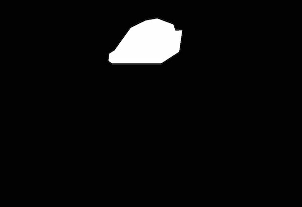
Here we have multiresolution blending using an irregular mask. We can see that it didn't blend too well. The background of the second image had very different intensities from the background of the first image when both were in gray scale. (See the section on Poisson blending to find out how these two images blended together using that technique).
For this part of the assignment, we explore the use of gradient-domain processing in order to blend images together seamlessly. We use least squares to solve this problem with blending constraints from our gradients.
We computed the x and y gradients of our image by creating a sparse matrix, A, and solving for x * y variables, using 2 * (imh * imw) + 1 constraints. Each variable we solved for is a pixel value in our output image. We had an additional constraint (the +1) for the upper left corner of the image.
Poisson blending is not too different from the algorithm we used for the toy image. However, now we have a source and target image. I created an A matrix of size target height * target width. If a pixel falls within the unmasked region, the pixel in the output will equal to the pixel in the target image. Thus, the corresponding variable's row in the A matrix would be like the identity matrix. If a pixel does fall within the masked region, then we have a more complex constraint and must calculate the summation of the differences between the pixel and its surrounding neighbors (left, right, up, down). We applied this algorithm for each channel in our colored images and then stacked the outputs to create our blended image.


Their skin tones are very different.
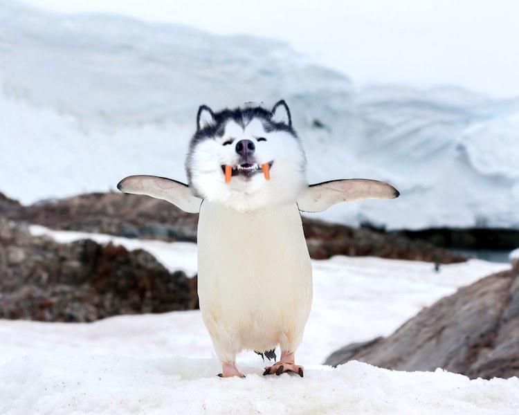
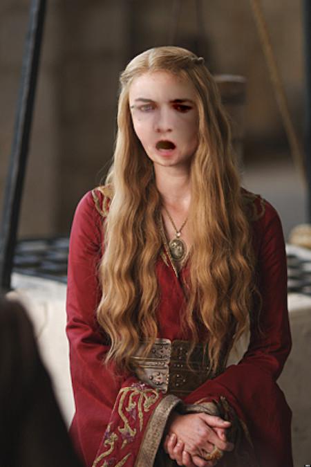
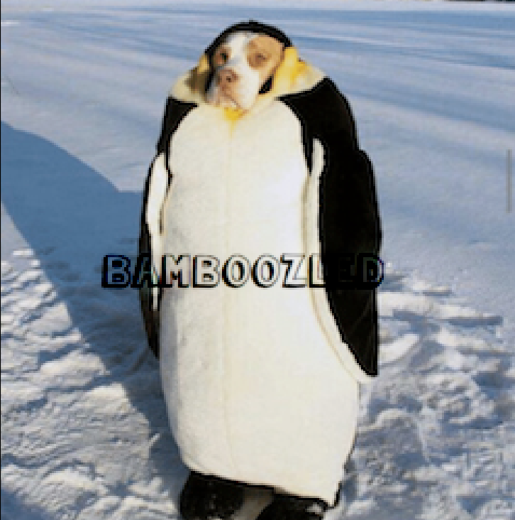
The Cersei/Joffrey image looks very warped because I had difficulty aligning the mask in the right position (especially using the Matlab code since we couldn't see the dimensions of the source image as we placed it on the target image). The Husky/Penguin picture also looks a bit off, not because it didn't blend well, but because the colors of the Husky didn't match great with the penguin's body. The bottom of the head of the husky is a little blended with the color of the penguin's body, but the top of the husky's head looks closer to the color of the mountain since the mountains are right behind the top of its head.
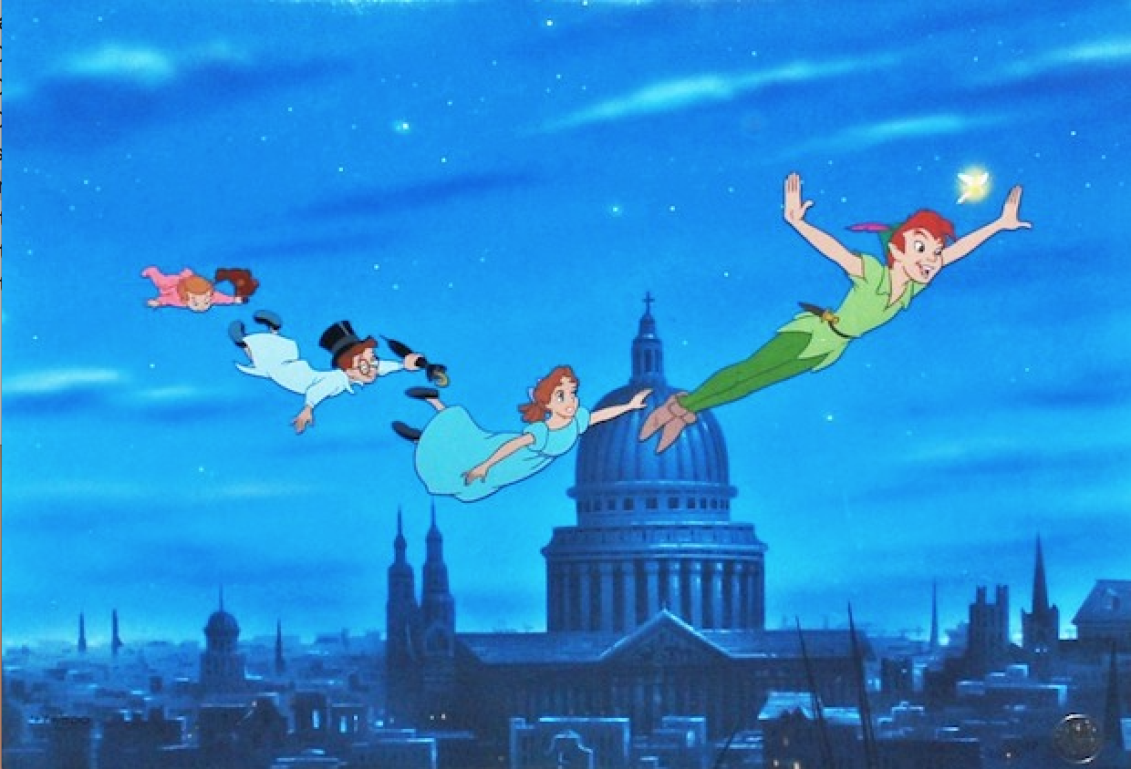
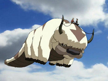
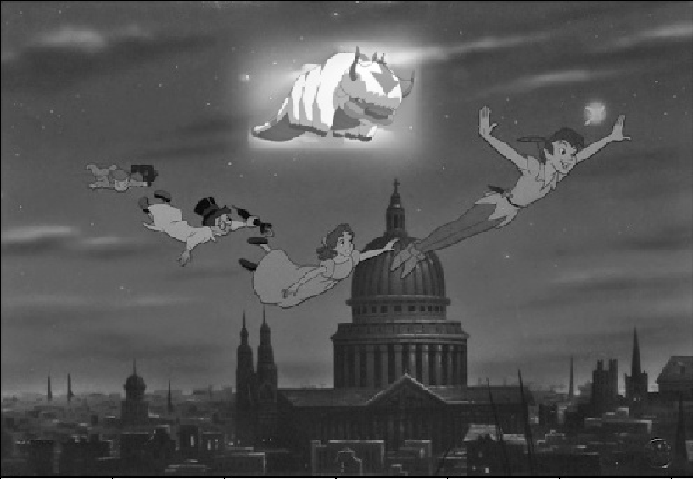
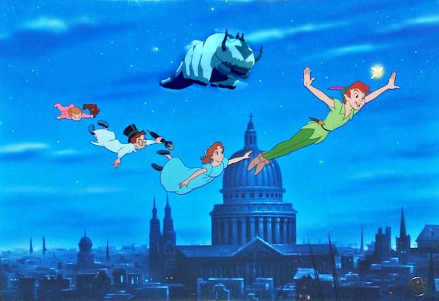
Revisiting the blending of Appa in the sky with Peter Pan: We have the Laplacian technique on the left and Poisson on the right. Poisson blending definitely created a more seamless blend compared to the Laplacian technique for the irregular mask. However, we also notice that Appa is a lot more washed out in the second image, so Laplacian works better if we want to preserve the colors of our source image and the two images align well.
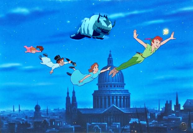
I also included the output for when I use the mixed gradients technique (more on this below). It doesn't look too different from the original Poisson blending.
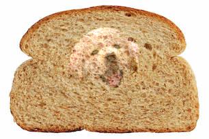
For normal Poisson blending, we used the source gradients to find the pixel in our output image that falls in the masked area. With mixed gradients, we compare the source gradient with the target gradient and use the gradient with the larger magnitude to solve for our pixel.

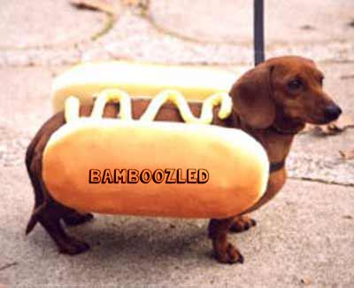


We saw in the Peter Pan / Appa image that using the source gradients in poisson blending vs. mixed gradients weren't too different. Here, I have two images, where the one on the left uses just the source gradients to construct the masked area, whereas on the right, the blended image is used using the mixed gradients technique. With mixed gradients, the pupper's face gets mixed in with the texture of the bread!