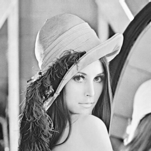
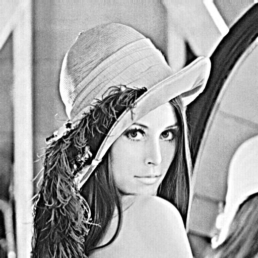
Here I used the unsharp technique to sharpen an image. For the unsharp technique, you create a high pass filter by blurring the image $f$ with a gaussian filter, then subtracting the result from the original image: $f - f \ast g$. The high frequencies are added back to the original: $f_{sharp} = f + \alpha(f - f \ast g)$. I chose $\sigma = 5$ for the Gaussian and $\alpha = 1$.
| Original | Sharpened |
|---|---|
|
|
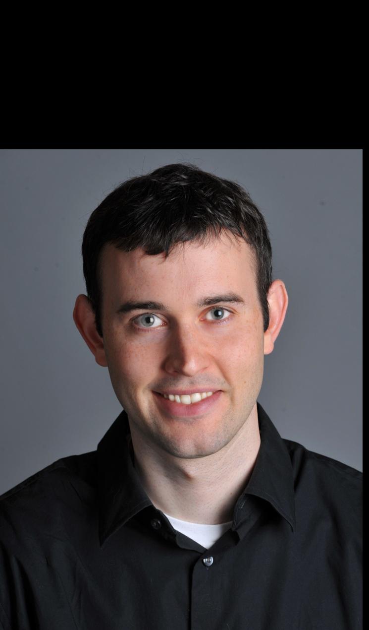
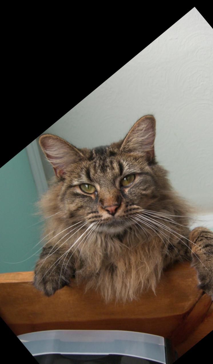
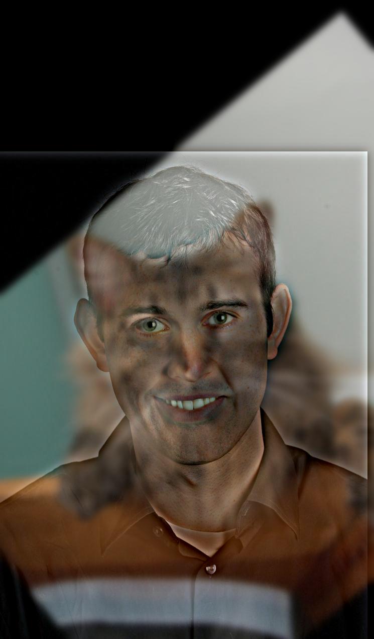
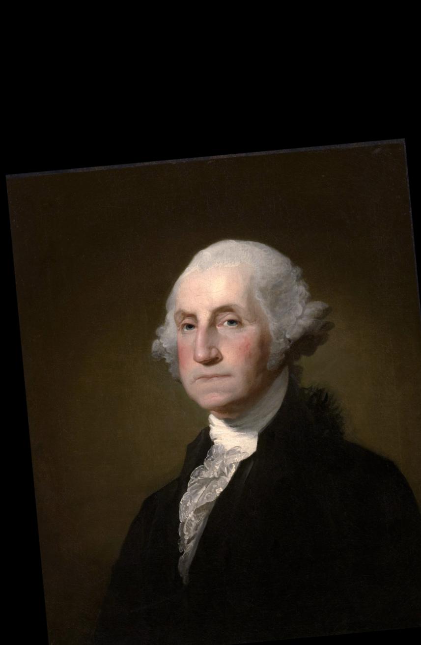
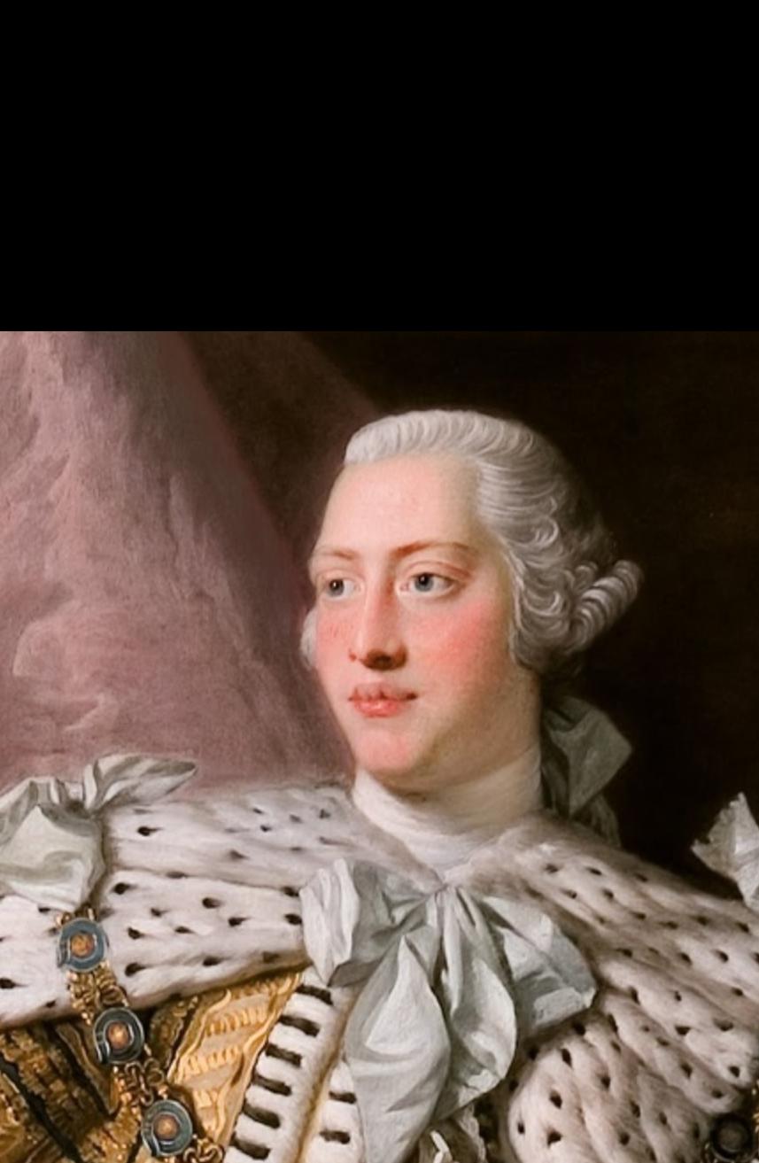
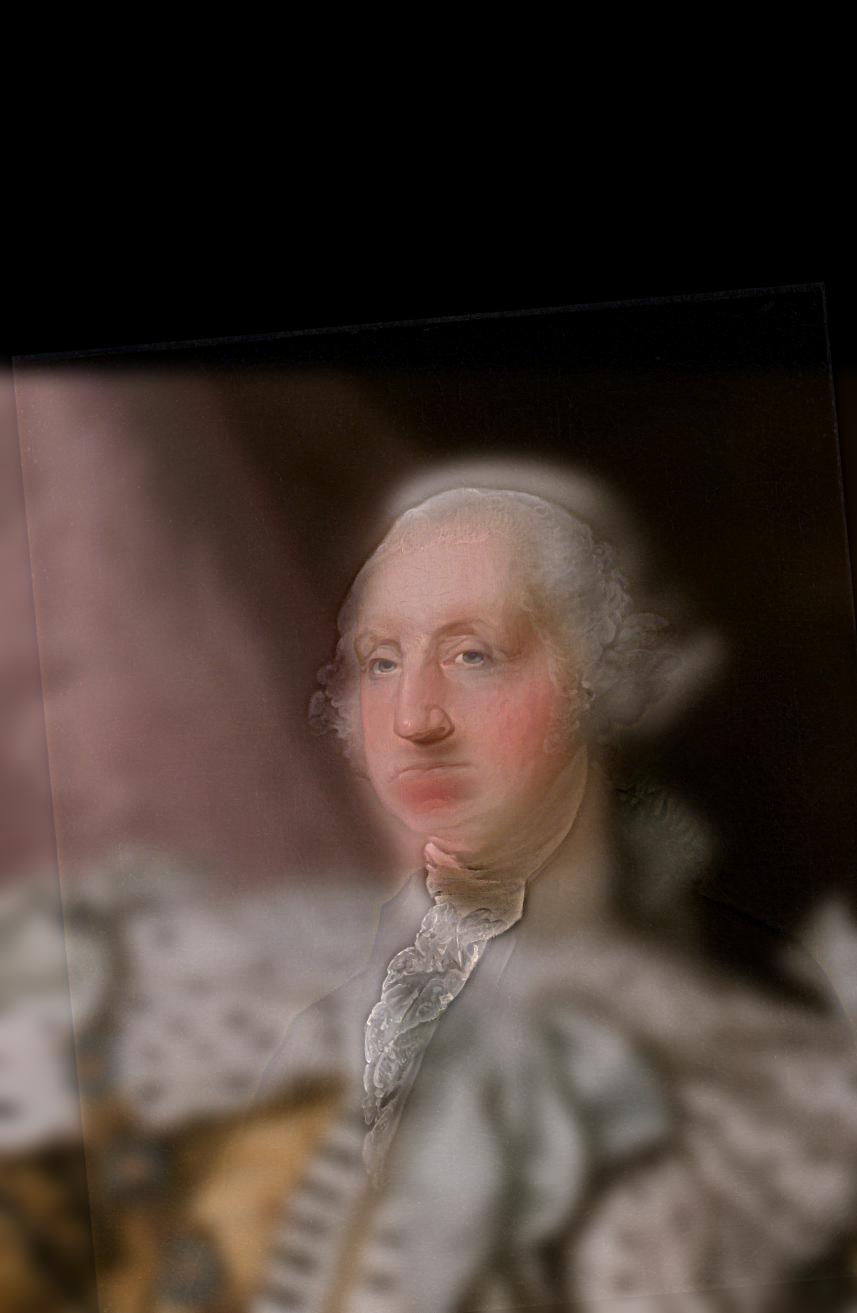
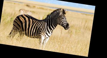
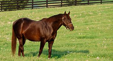
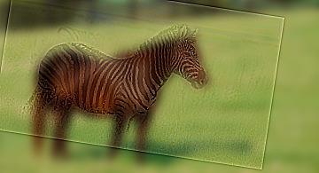
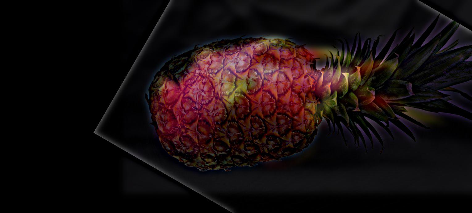
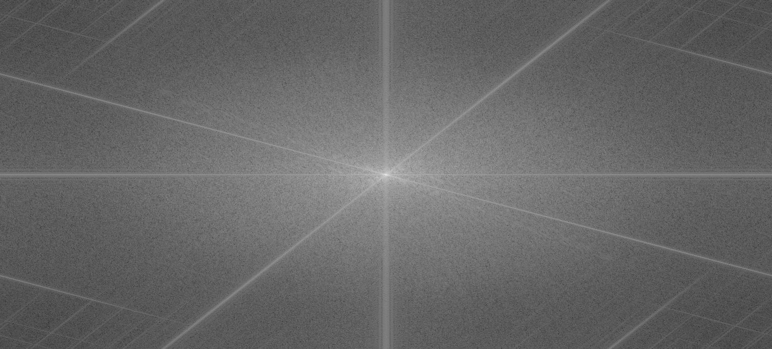
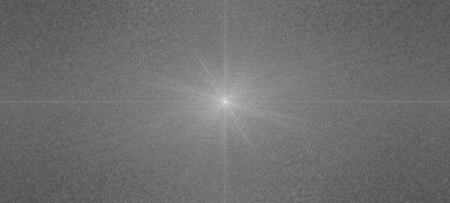
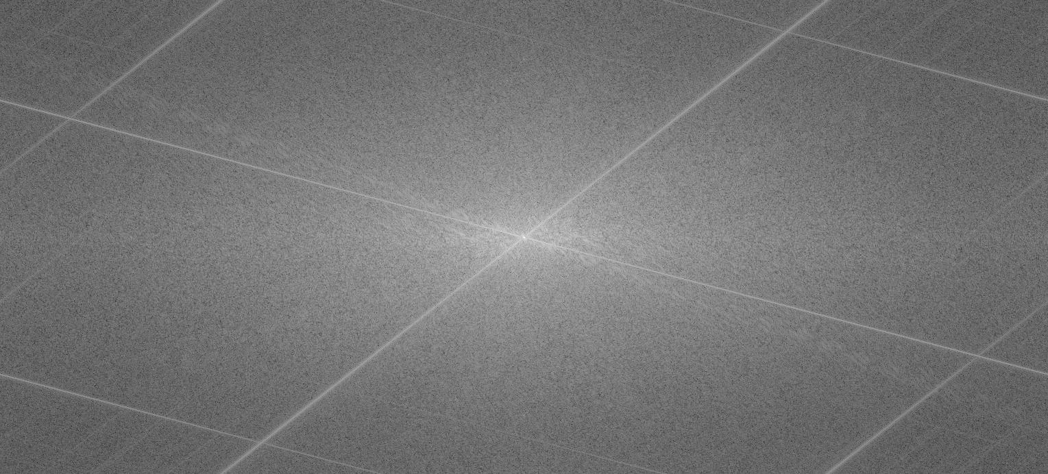
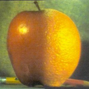
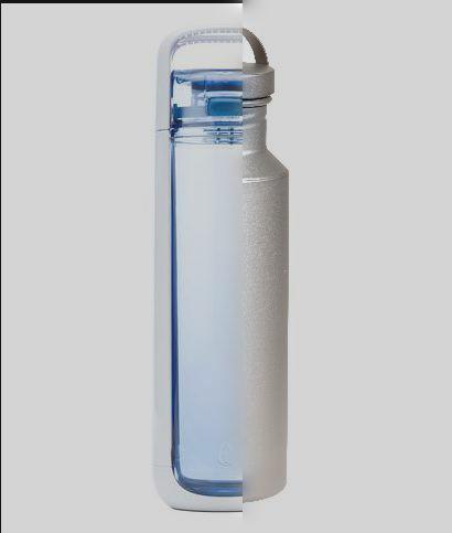
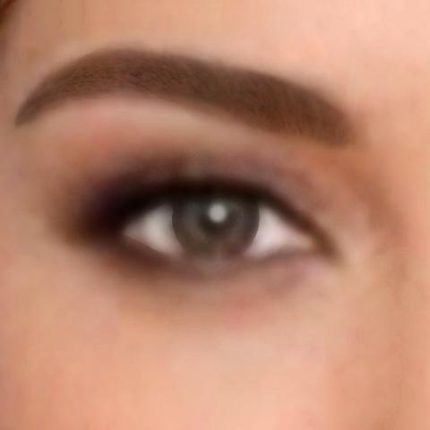
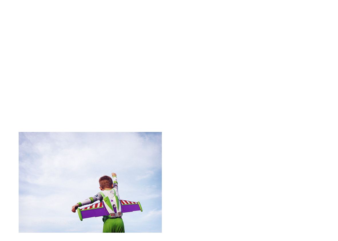
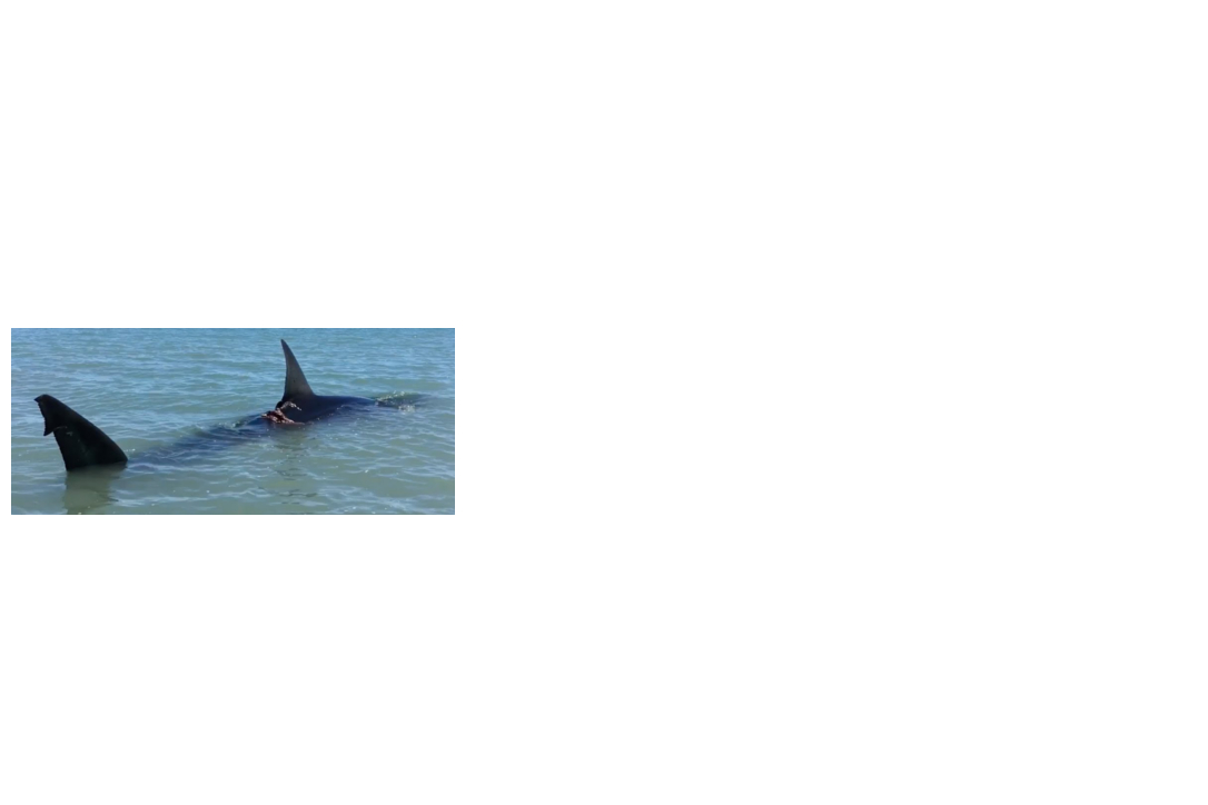
Hybrid images are created by combining the high frequencies of one image with the low frequences of another image. This requires high pass filtering the first image (as described in 1.1) and low pass filtering the second image (Gaussian blur). The two filtered images are then averaged to produce the hybrid result. Mathematically, $f_{hybrid} = 0.5 * (f_1 - f_1 \ast g_1) + 0.5 * (f_2 \ast g_2)$. Each Gaussian filter has a $\sigma$ that varies depending on the input images, and was chosen experimentally.
| High Freq Input | Low Freq Input | Hybrid Output |
|---|---|---|
 |
 |
 |
 |
 |
 |
 |
 |
 |
 |
 |
 |
| High Freq Input (pre-filter) | Low Freq Input (pre-filter) | High Freq Input (post-filter) | Low Freq Input (post-filter) | Hybrid |
|---|---|---|---|---|
 |
 |
 |
 |
 |
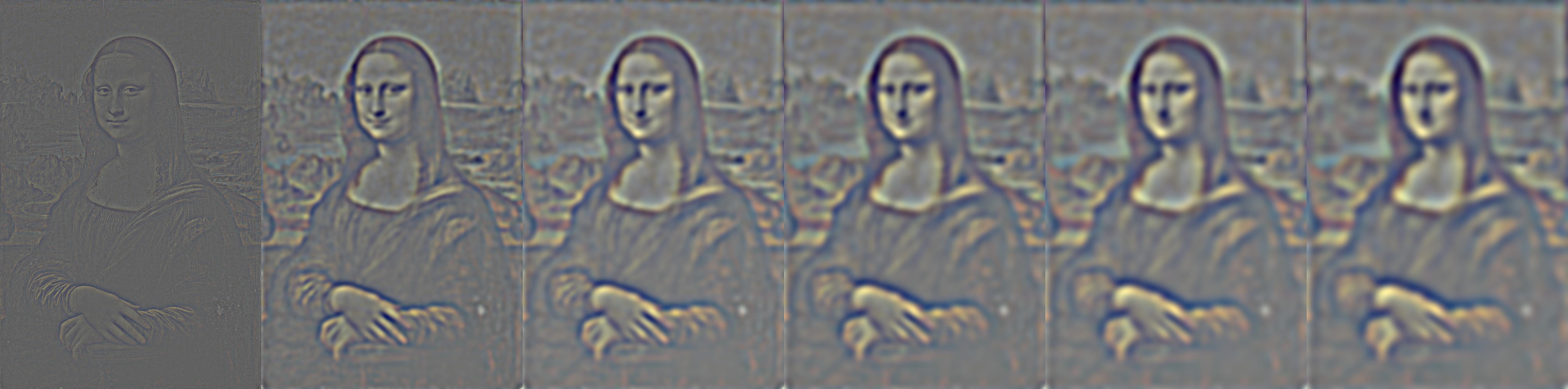
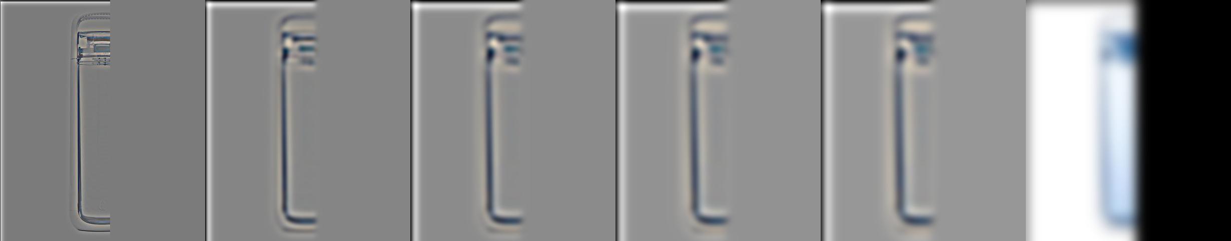
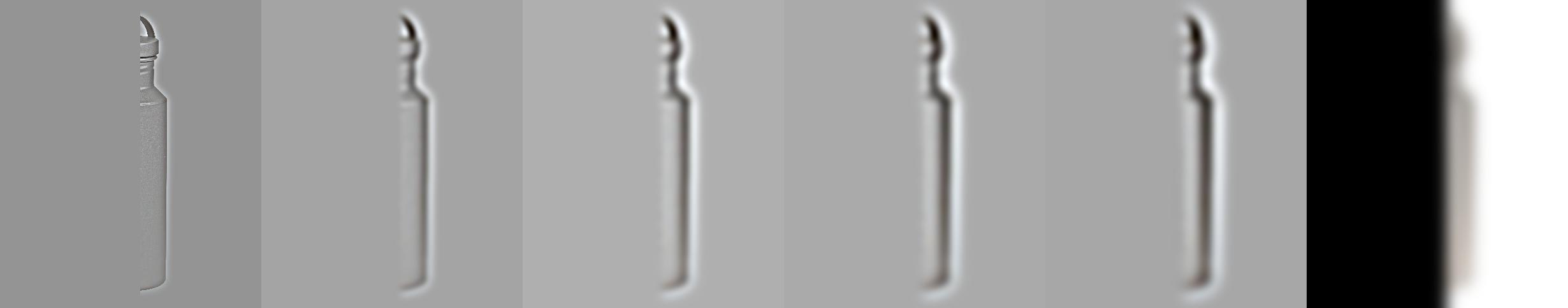
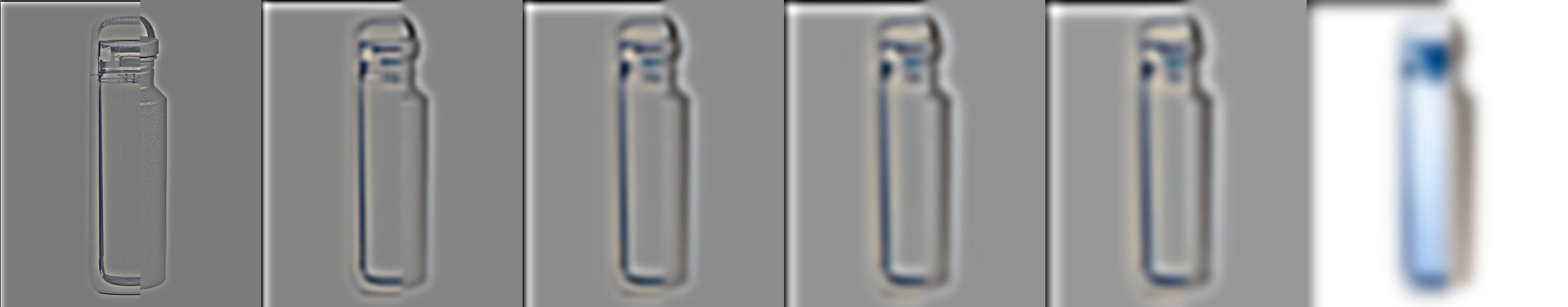
The Gaussian stack is created by applying Gaussian blur to the input image, then blurring the result, and so on for each level. The Laplacian stack is created by taking the difference between neighboring layers in the Gaussian stack.
 |
 |
 |
 |
 |
 |
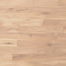
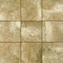
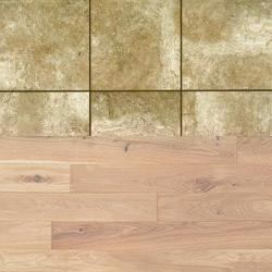
I use the Gaussian and Laplacian stacks for multiresolution blending, with 2 images $f_1,f_2$ and a mask $m$. To do multiresolution blending, I first construct the laplacian stacks for each image, and the gaussian stack of the mask. Then I combine the stacks to make a single output stack, which I sum up to produce the output Here, the laplacian stack for each image needs to contain the last image from the gaussian stack of that image, otherwise summing up the stack would not produce the original. Mathematically, $$f_{blend} = \sum_i \left(GStack_i(m) * LStack_i(f_1) + (1-GStack_i(m)) * LStack_i(f_2)\right)$$
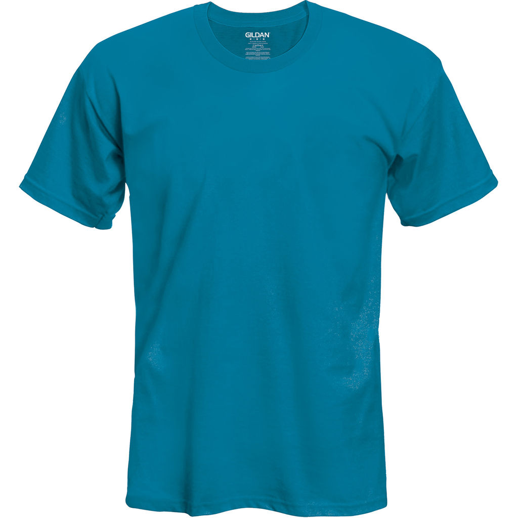
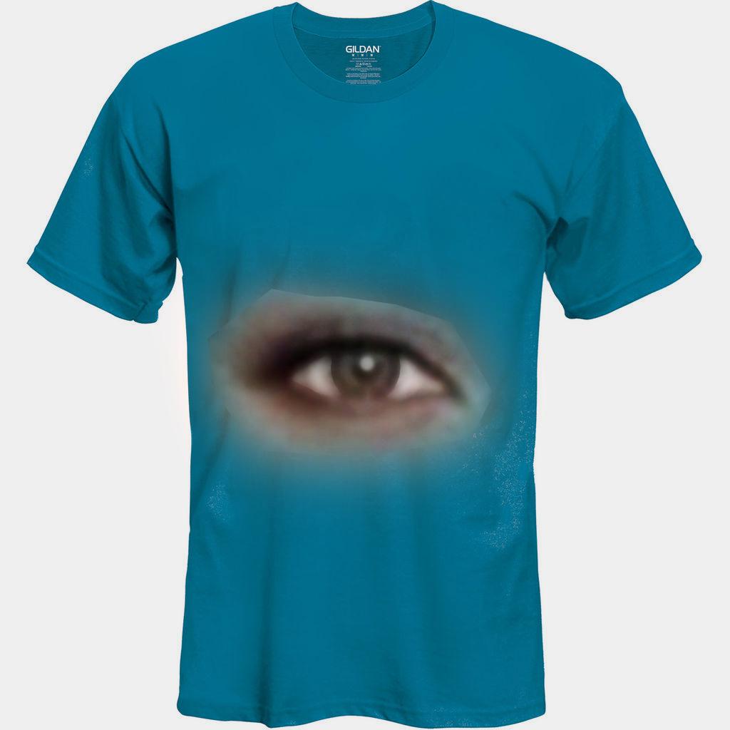
| Image 1> | Image 2 | Blended |
|---|---|---|
 |
 |
 |
 |
 |
 |
 |
 |
 |
 |
 |
 |
 |
 |
 |
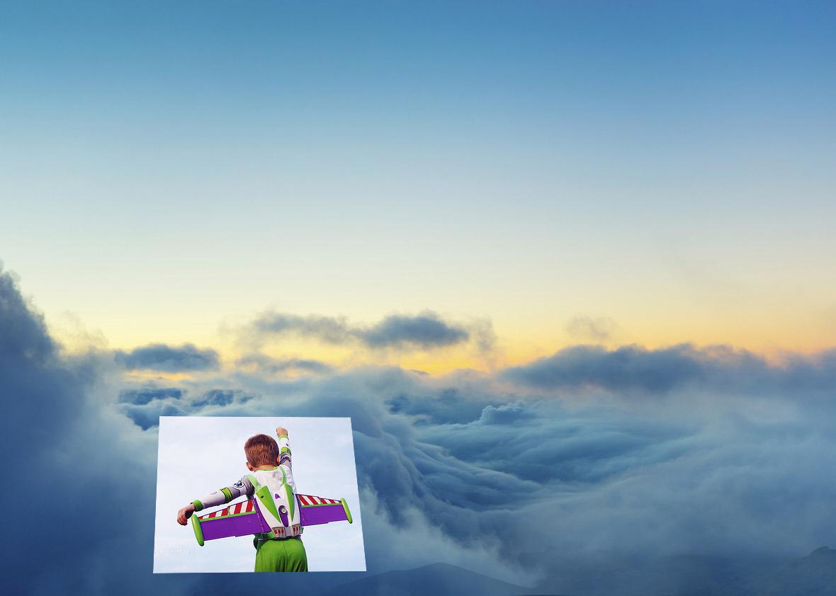
In this part of the project I do gradient domain fusion, which is another way of putting together images that tries to preserve gradients (rather than using frequencies for example). This is done by setting up a least squares minimization problem, where the optimization variables are the output pixels and the objective is to match the source gradients, with a constraint to enforce matching the source at the boundary (also, pixels outside the boundary should just match the target). Since the gradient is linear, you can set this up as a linear system $Av = b$ which encodes the gradient operations and constraints, then use existing linear system solvers/optimizers to recover $v*$ (the output).
For the toy problem, I set up a linear system $Av=b$ with sparse tall rectangular $A \in \mathbb{R}^{(2(h-1)(w-1)+1) \times hw}$. Each column of $A$ and entry of $v$ corresponds to a pixel $(x,y)$, and each row encodes objective terms in the least squares minimization problem (I fill in the matrix row by row for each term in the minimization problem). I then use a sparse matrix least squares solver to find $v^*$, the optimal result. Since each pixel not on the bottom or right edge has an $x$ and $y$ gradient, that contributes $2(h-1)(w-1)$ rows from gradient terms. The final row comes from the term $(v[0,0] - I[0,0])^2$ (top-left corner should stay the same). Solving this problem should just give back the original image.
| Original input | Reconstructed output |
|---|---|
 |
 |
This is really similar to the previous part, but I use a different definition of the gradient as given by the Laplacian filter: $$\Delta = \begin{bmatrix} 0 & -1 & 0\\ -1 & 4 & -1\\ 0 & -1 & 0 \end{bmatrix}$$ This means there is now just a single gradient term in the objective for each pixel in the mask: $$((4v_{x,y} - v_{x+1,y} - v_{x-1,y} - v_{x,y+1} - v_{x,y-1}) - (I_s\ast\Delta)[x,y])^2$$ This corresponds to adding a row to $A$ with 5 coefficients: a single $4$ for $v_{x,y}$ and four $-1$'s for its neighbors. Then I add an entry to $b$ with value $(I_s \ast \Delta)[x,y]$. For pixels not in the mask, we want to match the target image. If $v_{x,y}$ is not in the mask, I add a row to $A$ with a $1$ for $v_{x,y}$ and an entry to $b$ with $I_t[x,y]$. Technically, this only adds a soft constraint that the pixels outside the mask match the target, but in practice this works well enough. The Laplacian filter approach seems to produce better output, and uses a smaller matrix $A\in\mathbb{R}^{hw\times hw}$.
In practice I also needed to first crop to the axis-aligned bounding box of the mask and do all the optimization on the cropped images, which greatly reduced the number of variables in the problem. The optimization output is then spliced back into the target image to produce the full output.
Additionally, because there are 3 color channels I had 3 different $b$ variables, and solved 3 separate optimization problems for each image before stacking the results back together.
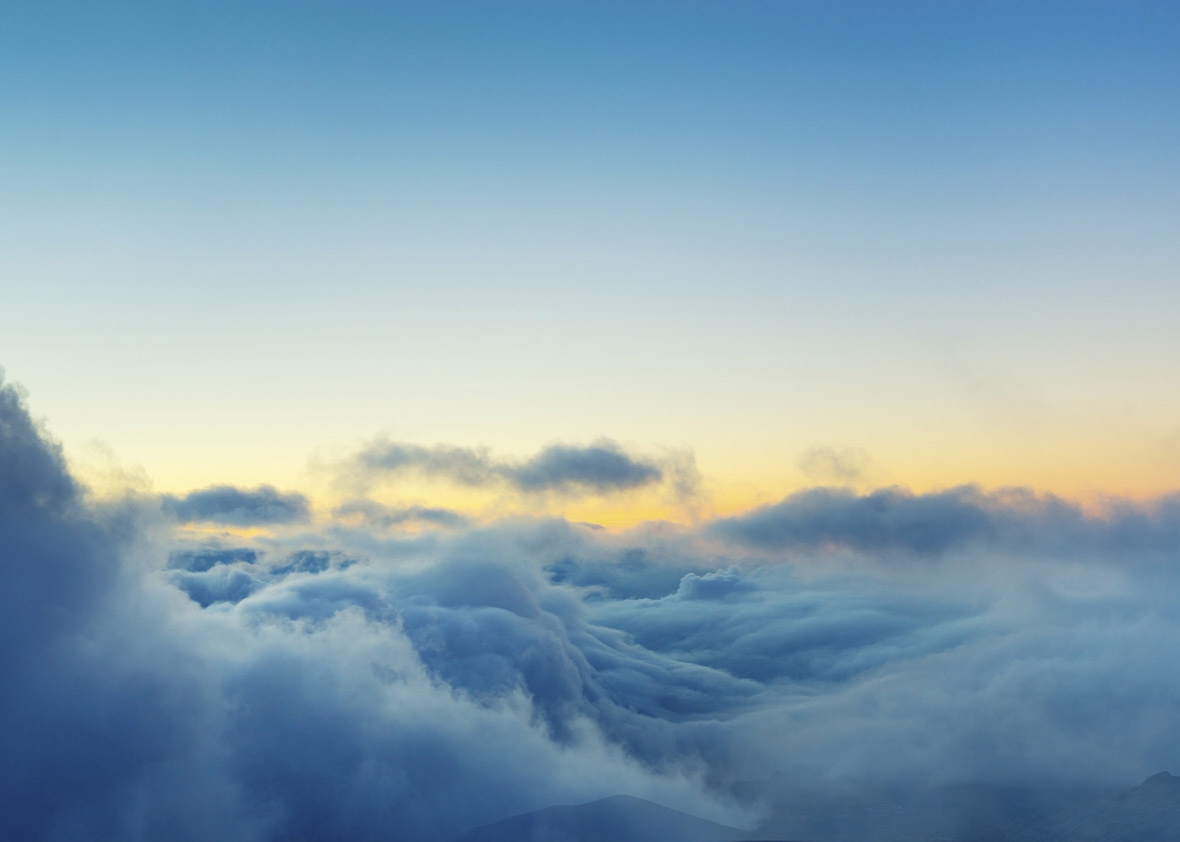
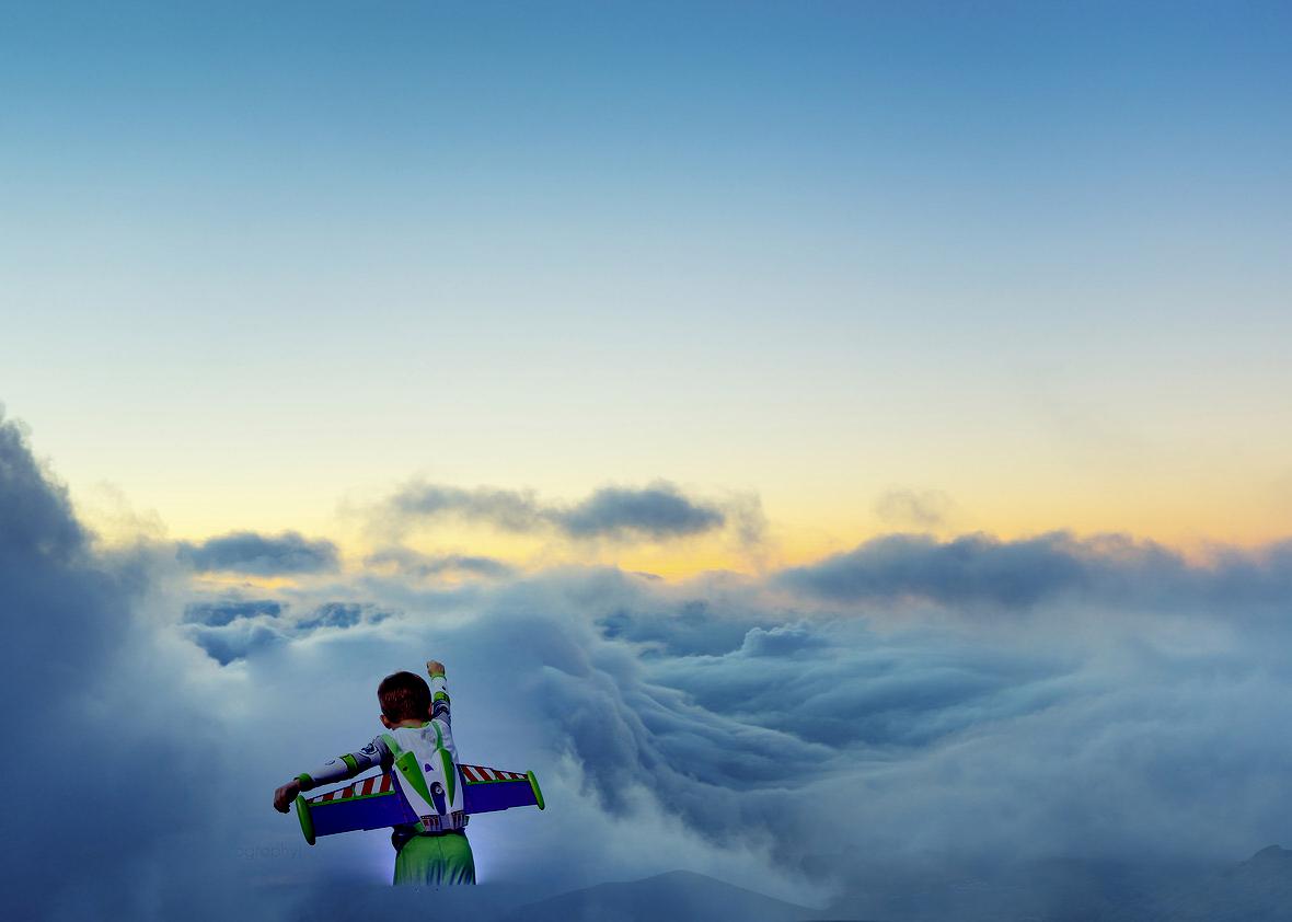
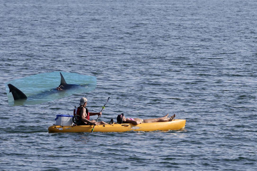
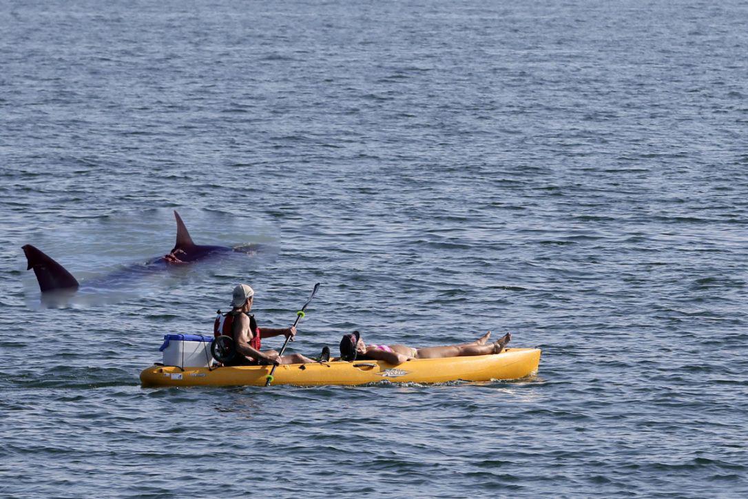
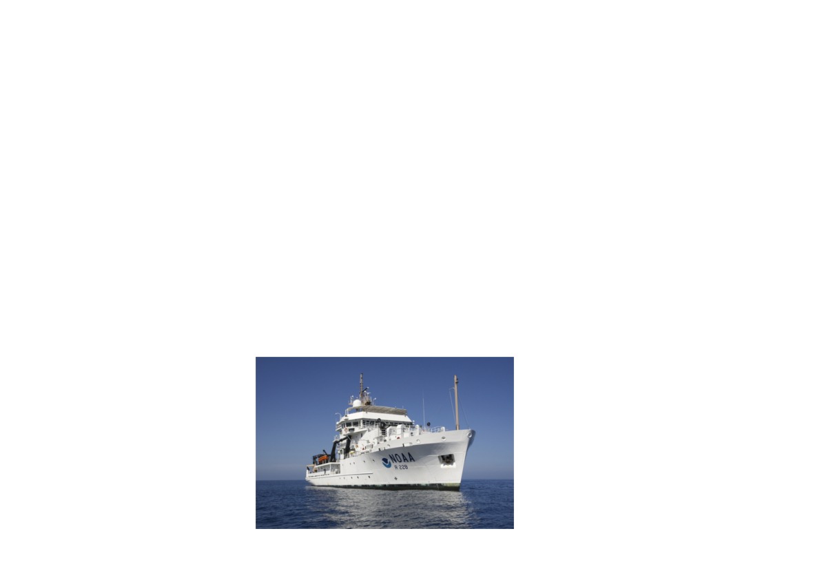
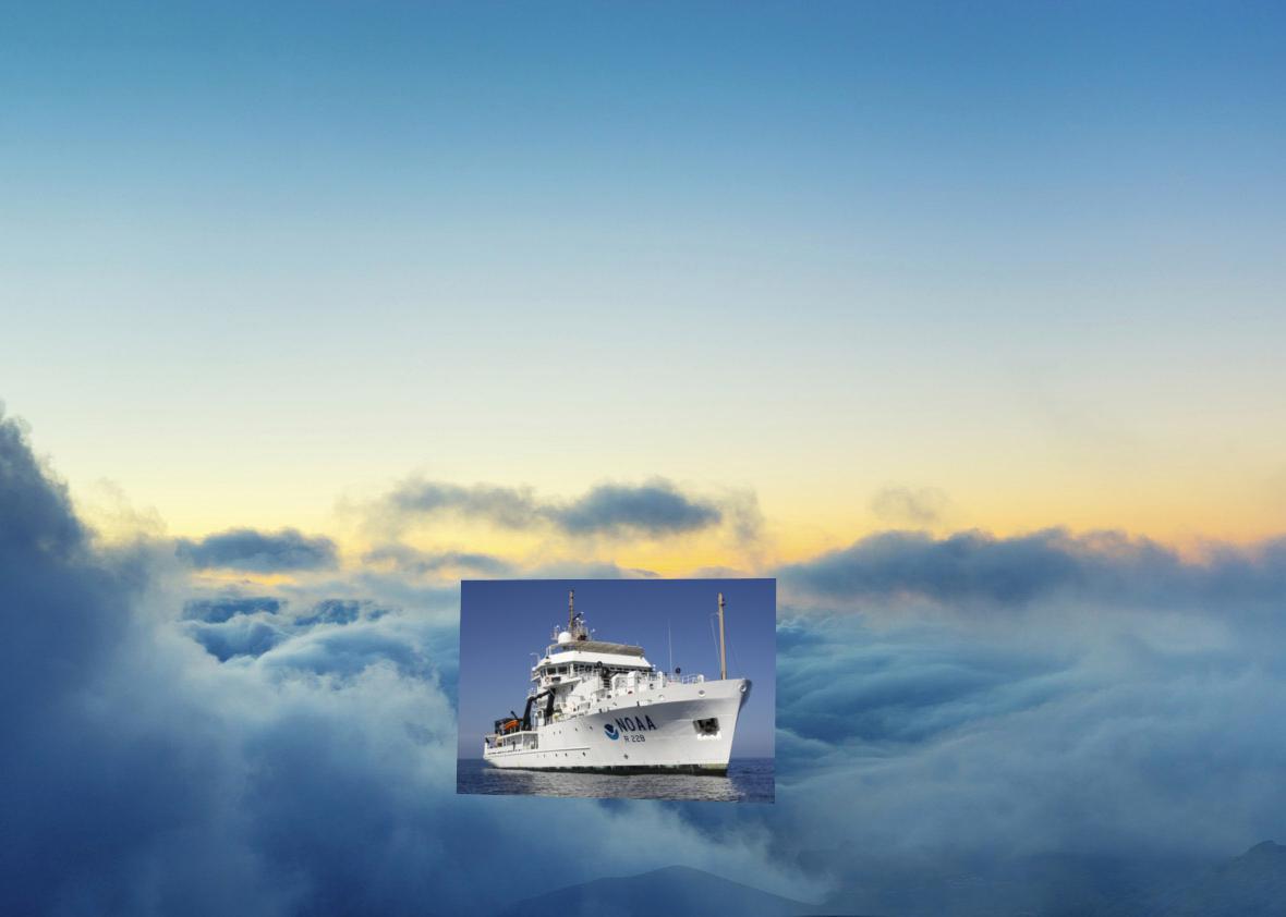
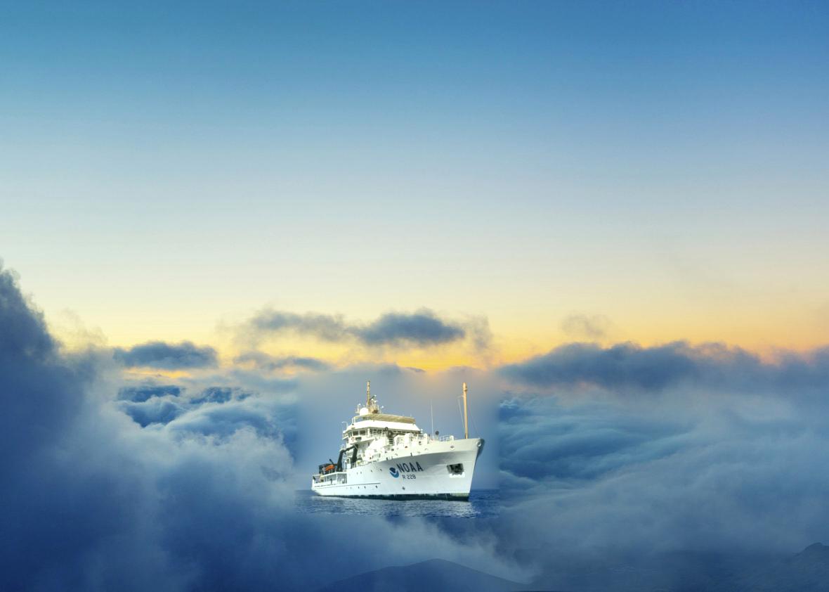
The difficulty of this approach is when the source and target have fairly different textures--for the final output with the ship in the sky it does a better job than naive but the result still doesn't look quite natural. I think this is because the clouds from the target image look quite different from the background in the source image.
| Target | Source | Naive Output | Poission Output |
|---|---|---|---|
 |
 |
 |
 |
 |
 |
 |
 |
|
 |
 |
 |
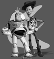
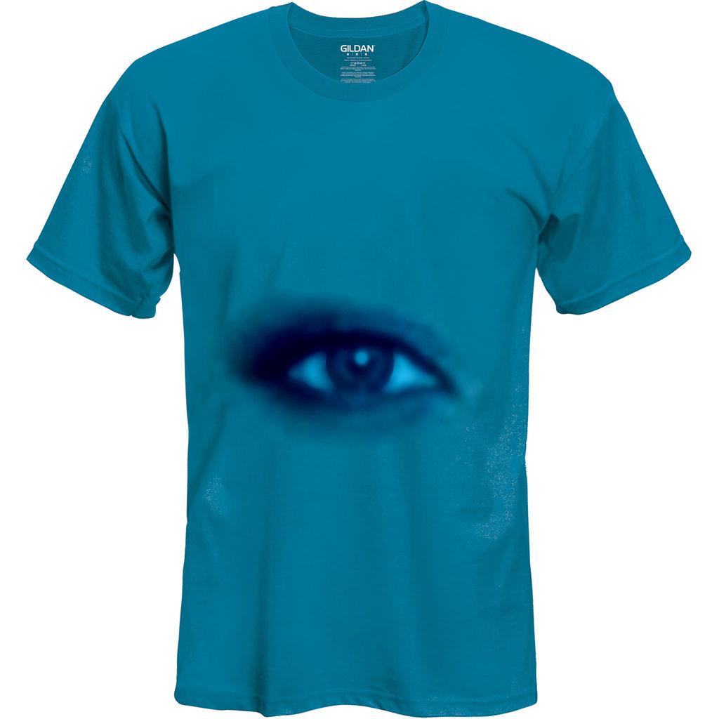
Here are the results from the multiresolution blending and the Poisson blending compared for the eye-shirt example. The biggest difference is that the Poisson output has a less noticeable seam, but also completely changes the color of the eye. This is because the Poisson blending is concerned with gradients, which makes it good at erasing the seam but makes it less concerned with color accuracy.
| Target | Source | Multires Output | Poission Output |
|---|---|---|---|
|
|
|
 |