CS194-26: Project 3
Fun with Frequencies and Gradients
Joseph Jiang
Part 1: Frequency Domain
1.1 Warm Up: Sharpening Images
To make images look sharper, we use a technique where we emphasize the higher frequencies of the image. In order to do this, we get the low frequencies of the image using the Gaussian filter. We subtract the low frequencies from the original image to get the high frequencies of the image. This higher frequencies are added to the original image to get the sharper image
Original Image
Sharpened Image
Low Frequencies
High Frequencies
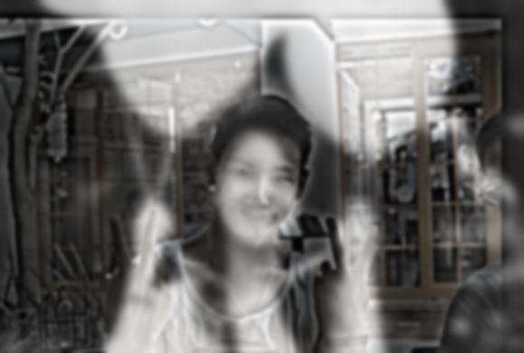
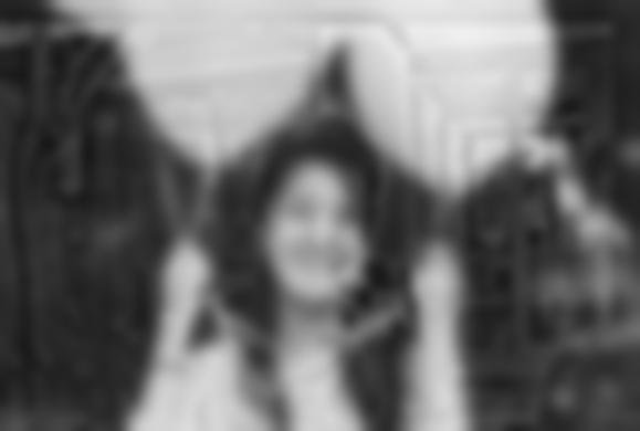
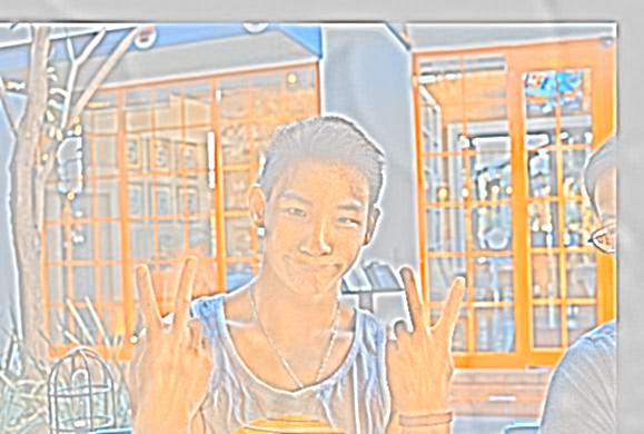
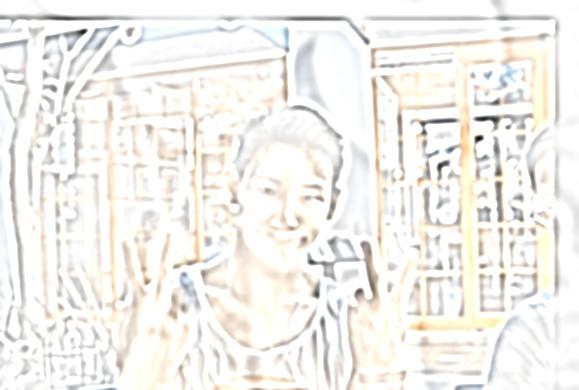
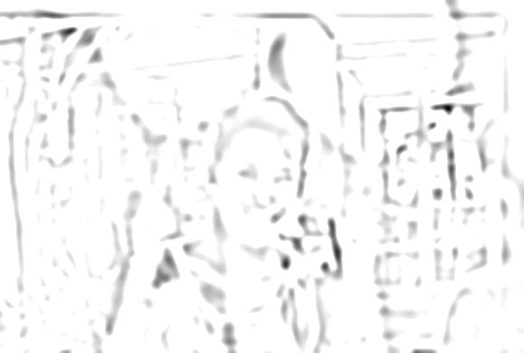
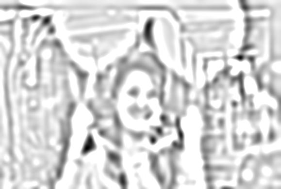
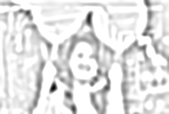
1.2 Hybrid Images
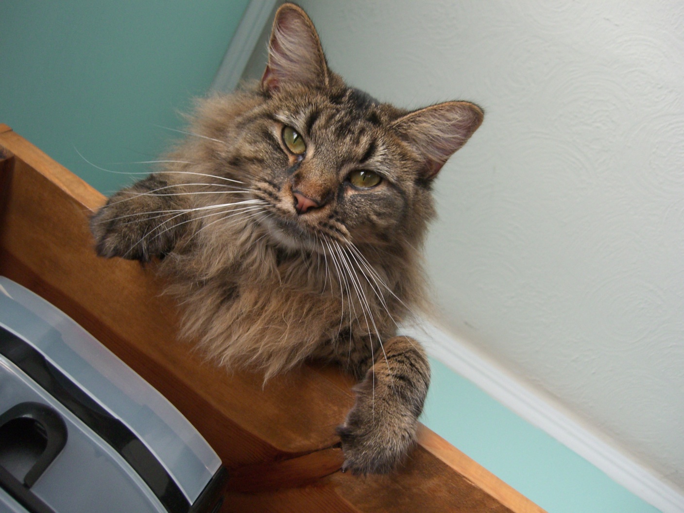
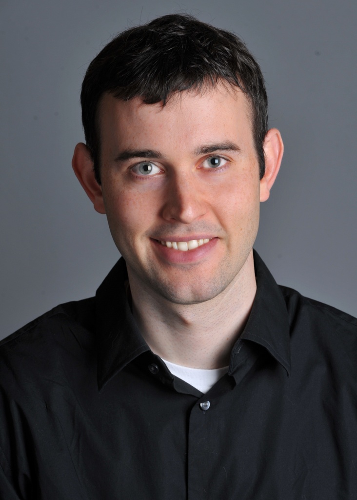
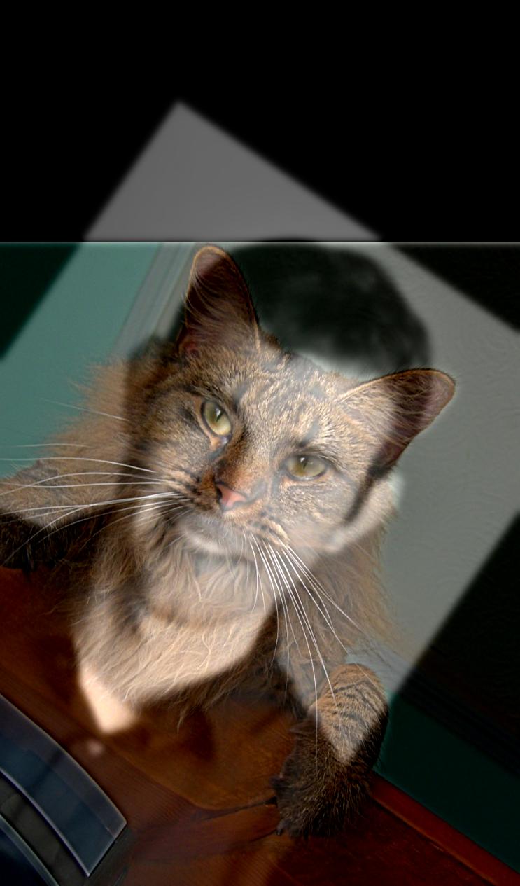
In this part, we created an static image that changes what it displays depending on the distance from the image. At closer distances, the high frequencies of an image dominates what a person sees, while, at a further distance, only the lower frequencies of the image are seen. This allows us to create images that display two images, a hybrid image.
Nutmeg
Derek
Hybrid
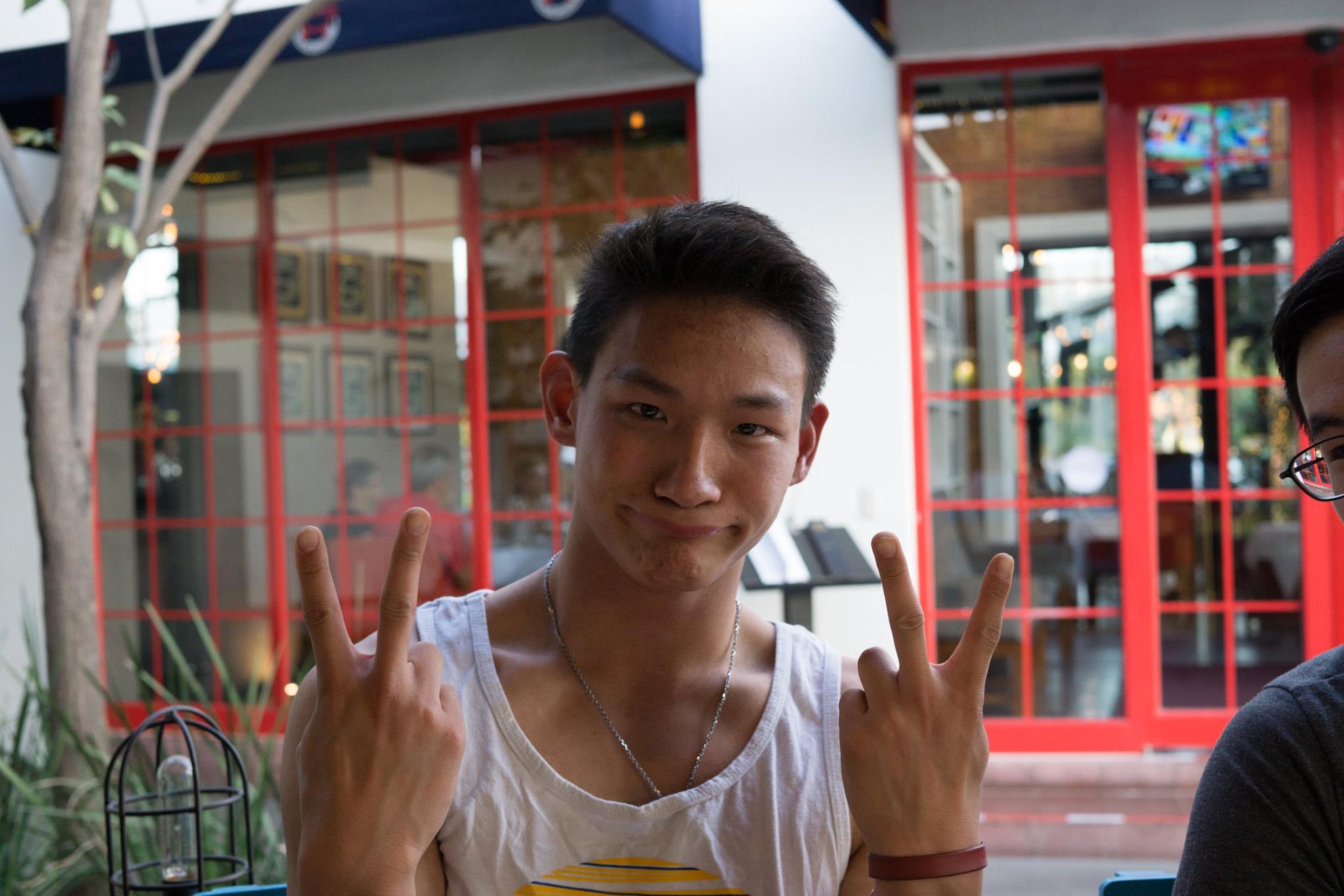
Joseph
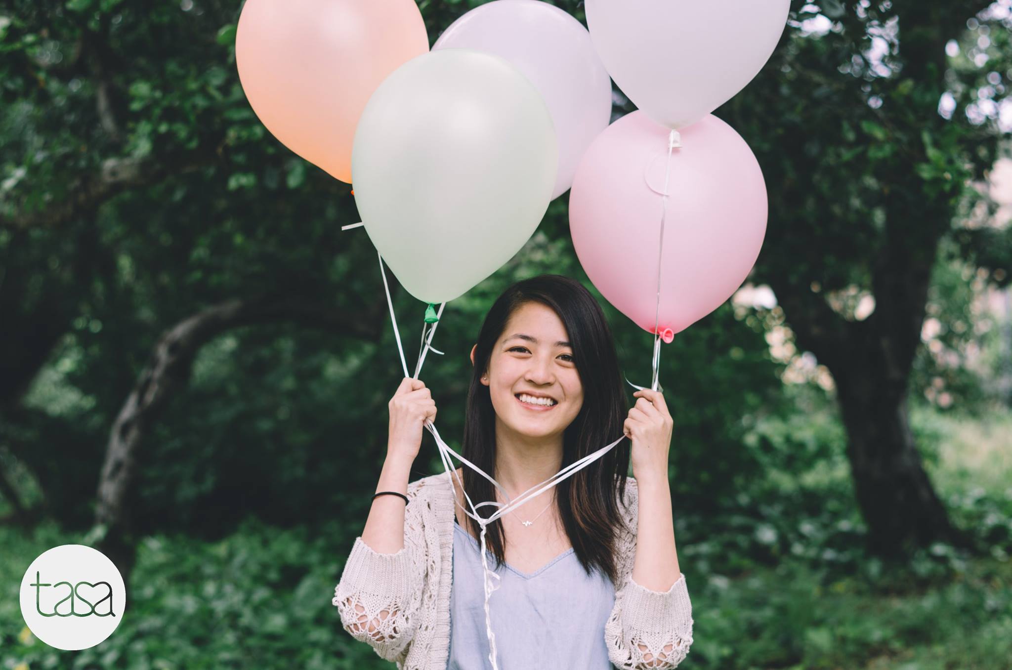
Katie
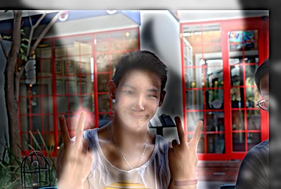
Hybrid
This failure is most likely due to the fact that Taylor Swift's image was photoshopped because certain colors were unnaturally bought out. For example, Taylor Swift's red lipstick stays in the image no matter what distance you view the image at.
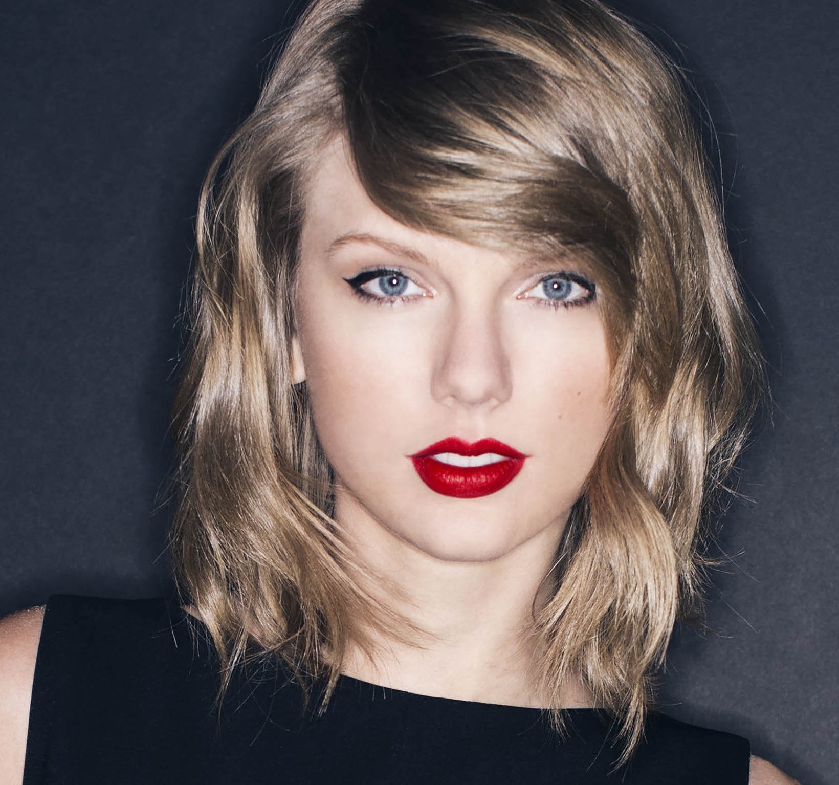
Taylor Swift
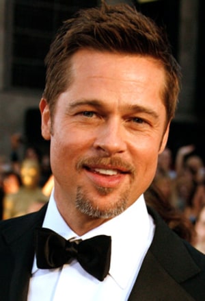
Brad Pitt
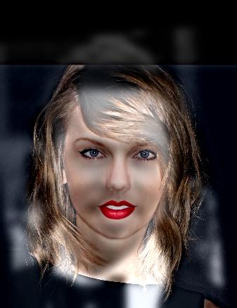
Hybrid
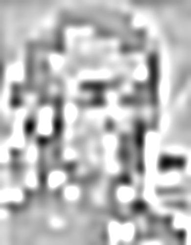
I analyzed the frequencies through the Fast Fourier Transformations of Joseph, Katie, High Frequencies of Joseph, Low Freqencies of Katie, and the hybrid image
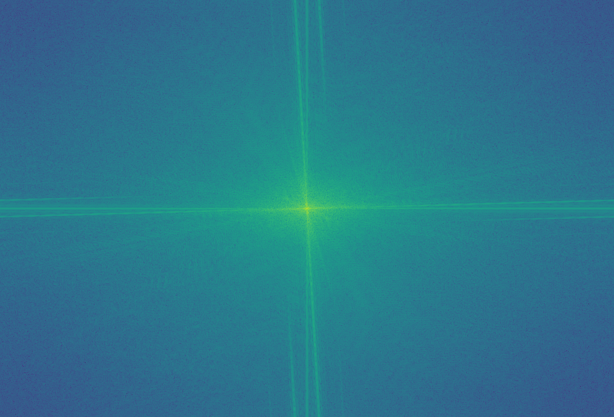
Joseph
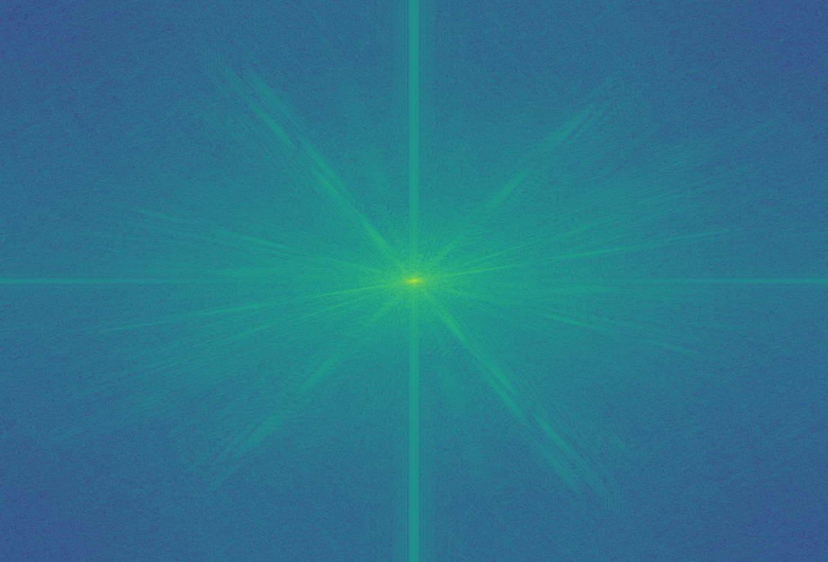
Katie
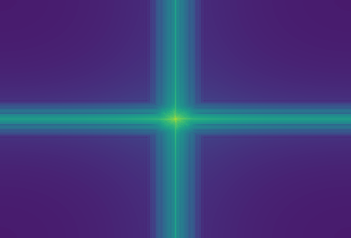
Low Pass
High Pass

Hybrid
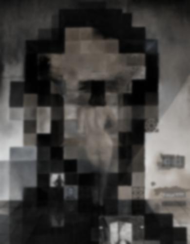
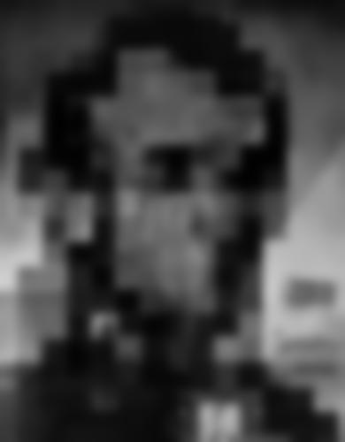
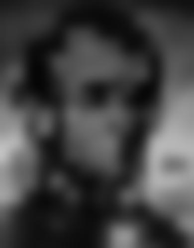
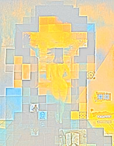
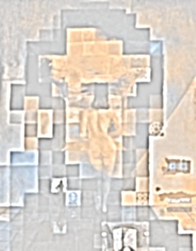
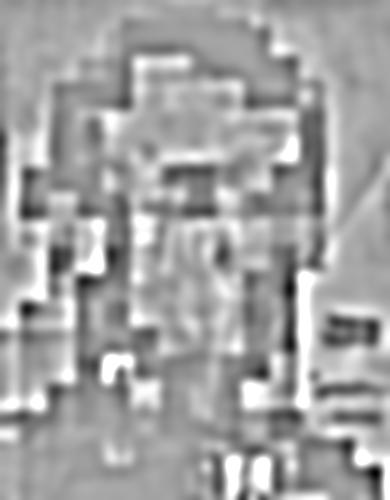
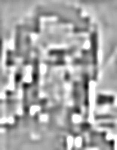
1.3 Hybrid Images
We needed to create a Gaussian stack and Laplacian stack so I chose to set the stack size to 5 and doubled the value of sigma for each level. The Gaussian stack simply consisted of gaussian filtered images produced through the use of the respective sigma value at that layer. The Laplacian stack was a little more difficult to create because each level was created through subtracting the previous layer's gaussian filtered image (low sigma value) by the current layer's gaussian filtered image.
Gaussian: Level 1

Gaussian: Level 2
Gaussian: Level 3

Gaussian: Level 4

Gaussian: Level 5
Gaussian: Level 6
Laplacian: Level 1
Laplacian: Level 2

Laplacian: Level 3
Laplacian: Level 4
Laplacian: Level 5
Laplacian: Level 6
Gaussian: Level 1

Gaussian: Level 2
Gaussian: Level 3

Gaussian: Level 4

Gaussian: Level 5

Gaussian: Level 6
Laplacian: Level 1
Laplacian: Level 2
Laplacian: Level 3
Laplacian: Level 4
Laplacian: Level 5
Laplacian: Level 6
1.4 Multiresolution Blending
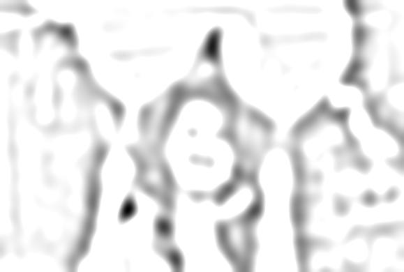
This part was slightly more involved then the previous parts. First, I used the same logic from part 1.3 to create the Laplacian stacks for the two images that I'm trying to blend. Then, I created the gaussian mask which, for the purposes of the apple and orange blend, is a matrix the size of the images that has all ones on one side and all zeros on another. Then, we passed it through a gaussian filter to blur the boundary.
Then, we need to blend the two images toegther at each level of the Laplacian stack so I calculated (mask * laplacian_image_1) + ((1 - mask) * (laplacian_image_2) for each level and, then, summed all the layers together to get my final blended image.
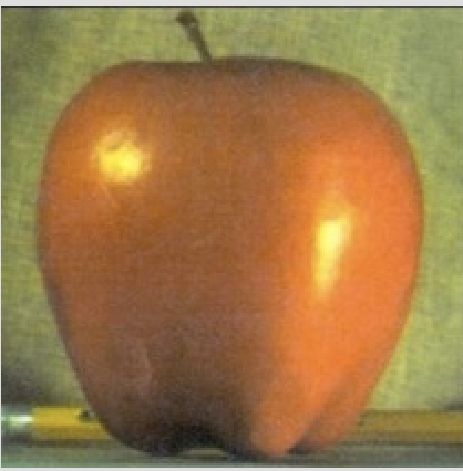
Apple
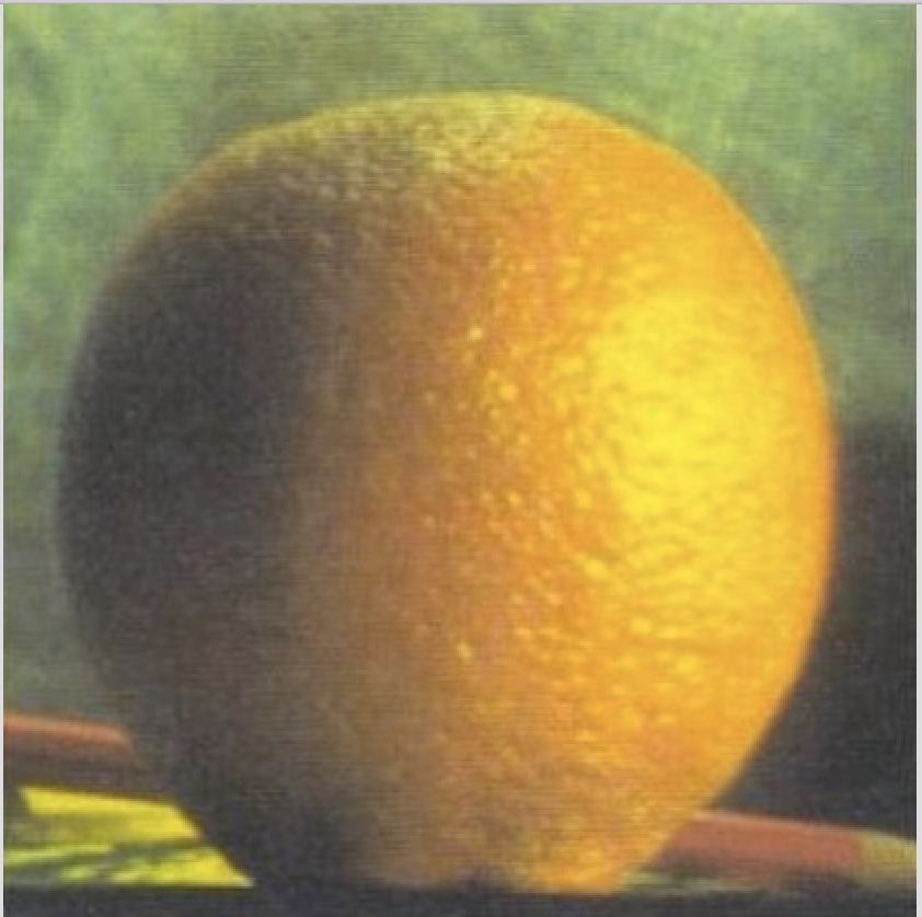
Orange
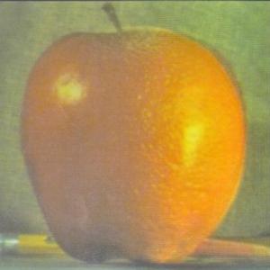
Multiresolution Blend
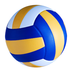
Volley Ball
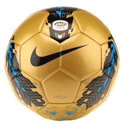
Soccer Ball
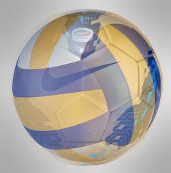
Multiresolution Blend
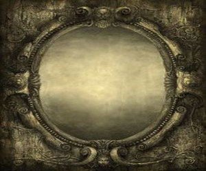
Mirror
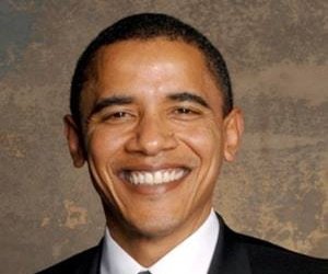
Obama

Multiresolution Blend
Part 2: Gradient Domain Fusion
2.1 Toy Problem
The problem was essentially setting up Ax = b and solving for x. We populated our matrix A with the three different objectives listed in the project spec. First, the x-direction gradients where (y, x+1) and (y, x), encoded to 1 and -1 respectively. Second, the y-direction gradients where (y+1, x) and (y, x), encoded to 1 and -1 respectively. Third, the top left corner was just hard coded in to we have a fully ranked matrix. Our B-vertex was populated by computing the result of the gradients at each pixel (for both x and y direction gradients). I. E. b[e] s[y, x+1] + -s[y, x].
Since matrix A had mostly zeros, I decided to use sparse matrix (lil_matrix) to improve the runtime. Before solving for x, using least squares, I converted the lil_matrix to csr_matrix. Finally, solving for x gives us the values for the actual image itself (value v). Looping through the values of v, and copying it onto a matrix of the dimensions of the orginal image, you create the final image.

Original Image
Reconstructed Image
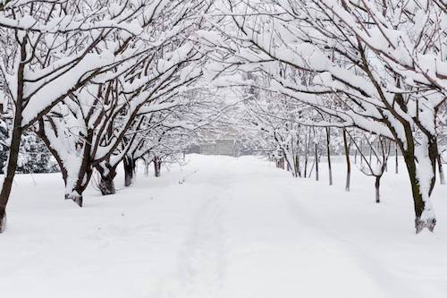
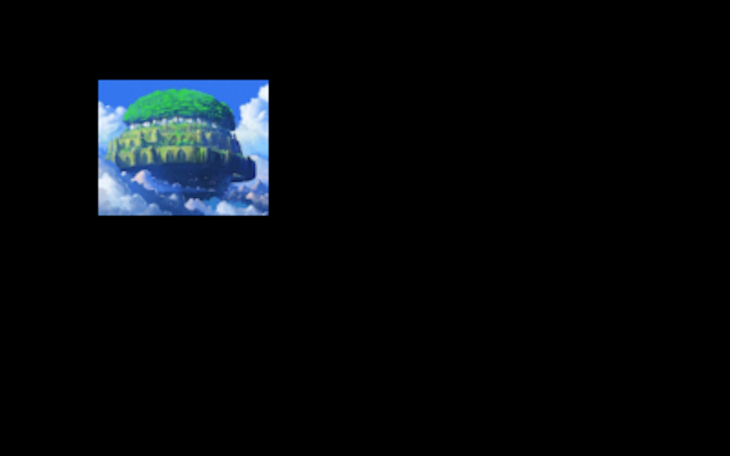
2.2 Poisson Blending
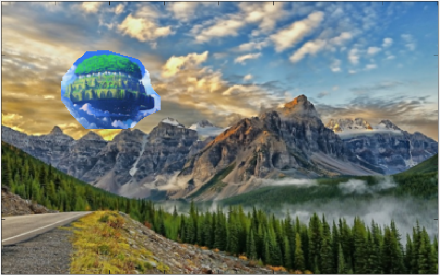
In this part, we seamlessly blend some object from a source image onto a target background. The naive solution to this problem is to directly copy and paste the source image object onto the target background. However, this gives us noticable seams between the original target background and the source object. In this part, we take advantage of the fact that human's notice the gradient of an image more than the actual overall intensity of the image. So we do not have to maintain the original color values but we can adjust so that it blends seamlessly with the background target. Our goal is to perserve the gradient of the source object without modifying the target image pixels.
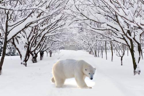
Polar Bear Blend
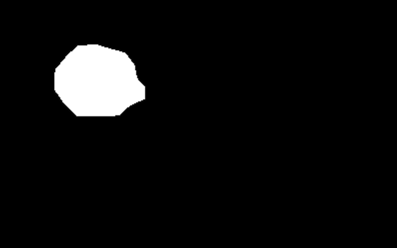
Implementation: Our goal is to create a target and source image to create a blended image. The first thing we needed to do is create a mask for the exact region in the source image we are blending with the target background. Next, we need to pre-process all the images (source, target, mask) so that they are all the same size. Finally, we use the least square method that we employed in the previous part 2.1 and find exactly what pixels will make our resulting image.
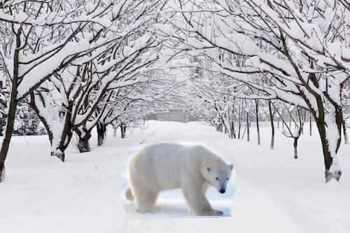
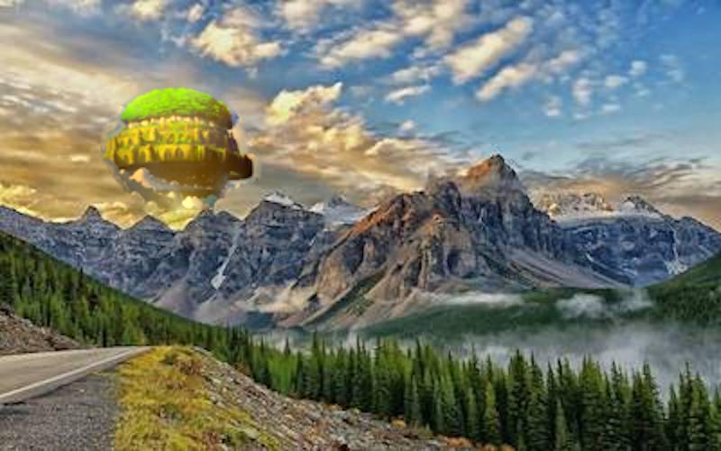
We essentially created a sparse Matrix A and vertex B so that we could solve the equation Ax = B for x. We populate Matrix A so that each row is a gradient comparison with the current pixel value within the mask and its 4 neighbors (up, down, left, right) within the mask. If the neighbor happens to be outside of the mask, then we take the pixel value from the target background. Then, we populate vertex B with the relative intensities from the neighboring pixels. This results in a seamlessly blending image.
Target
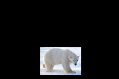
Source
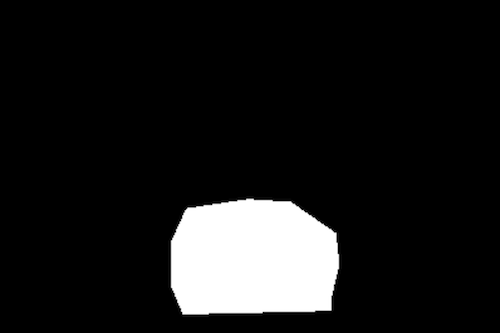
Mask
Naive Solution
Poisson Blend
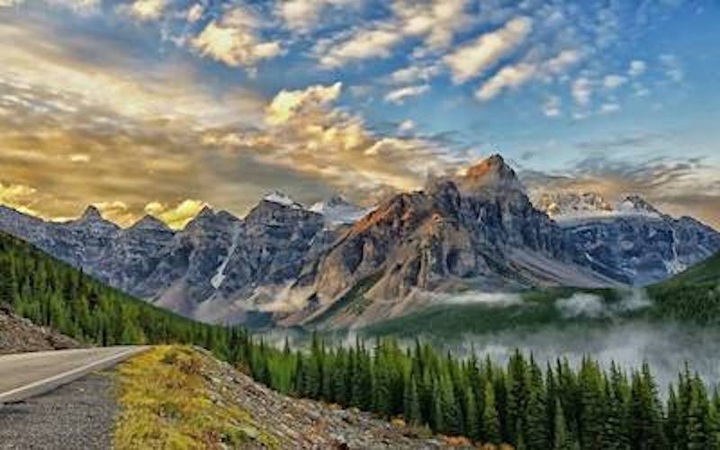
Target
Source
Mask
Naive Solution
Poisson Blend
Failures
The failure is due to the huge color changes nessesary for the source target object to undergo in order to satisfy the gradient from the target background. This results in dolphins that are red. This technique of blending relies on the fact that the color changes due to satisfying the gradients are unnoticable. However, this was not the case.
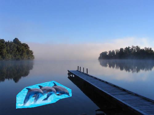
Naive Solution
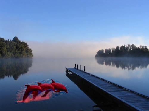
Poisson Blend
Comparison of Laplacian Blend vs. Poisson Blend
The poisson blend did a lot better than the Laplacian blend because the white space in the Obama's image screws up the Laplacian Blend.
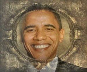
Multiresolution Blend
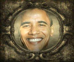
Poisson Blend