CS 194-26 Project 3
Fun with Frequencies and Gradients!
Quinn Tran (abu)
Part 1: Frequency Domain
Part 1.1: Warmup
I used the unsharpening technique from lecture to sharpen an image. Create a high pass filter by convolving image f with a gaussian filter to create a blurred image, then subtract the blurred image from the original image f: f - f * g. f_sharp = f + alpha(f - f * g).
Scene 1: Turtle
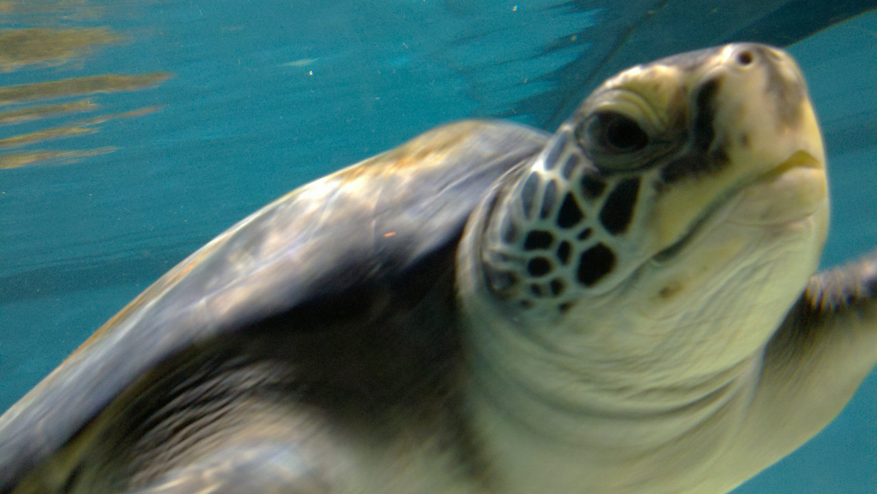
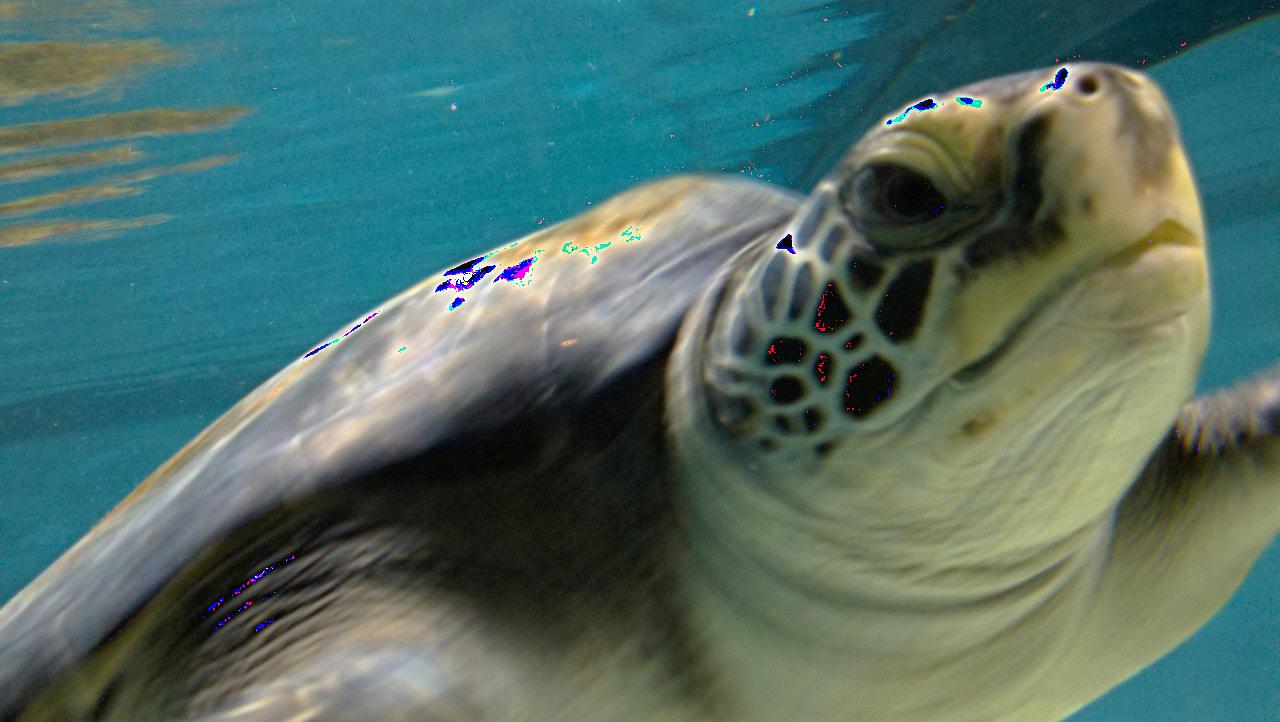
original, sharpened; alpha = 1, sigma=3
Part 1.2: Hybrid Images
Hybrid images were made by high frequencies of one image + low frequencies of the other image. We high pass filter image_1 (f_1) and low pass filter image_2 (f_2) like in the warmup. f_hybrid = (f_1 - f_1*g_1) + (f_2 * g_2). Proper alignment was extremely important. Images that weren't fully aligned (such as Derek and Nutmeg, didn't look completely "believable". sigma_im1 = 9, sigma_im2 = 2.5
Scene 1: DerekNutmeg/p>
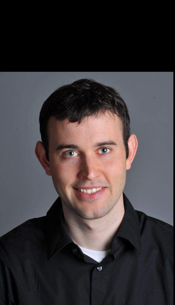
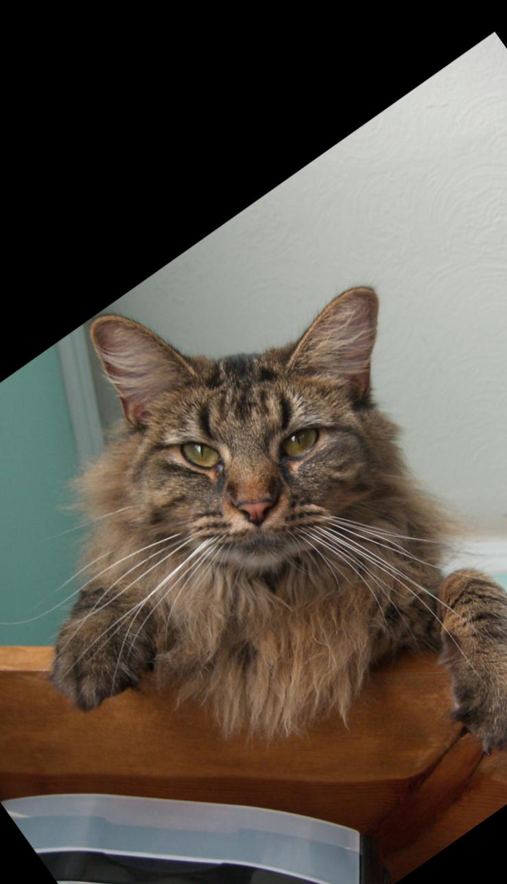
Derek, Nutmeg, DerekNutmeg
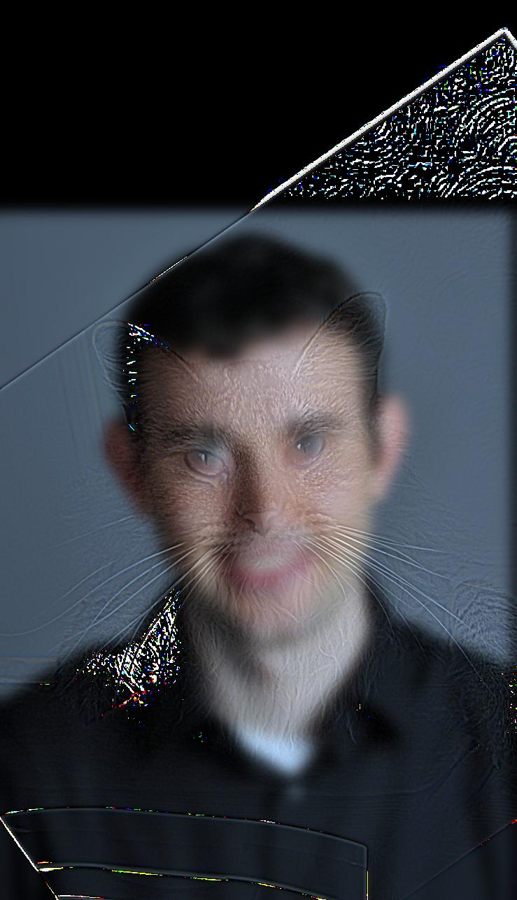
Scene 2: Catbread
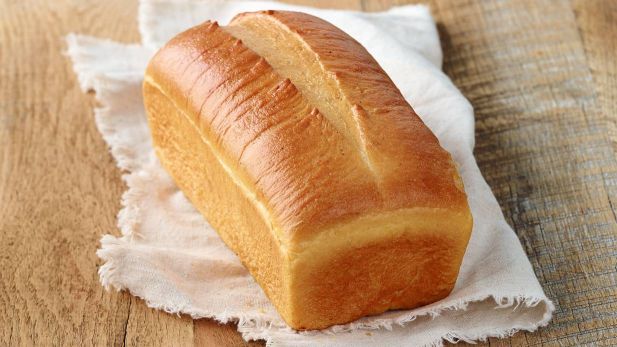
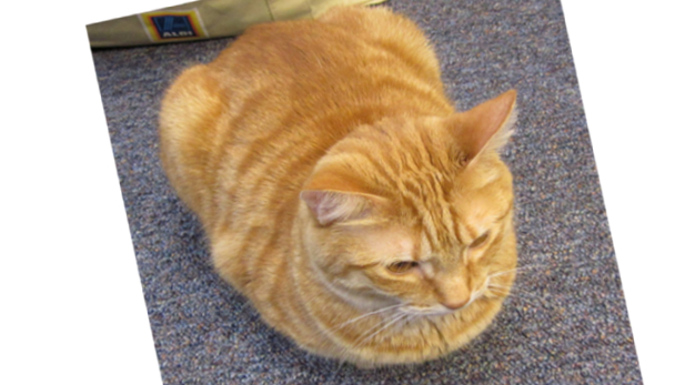
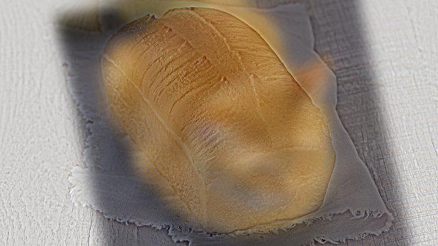
bread, cat, catbread
Scene 2: Albert Monroe
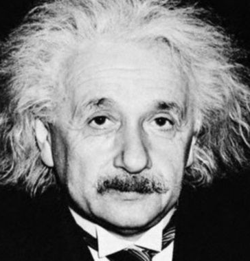
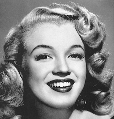

Einstein, Monroe, Albert Monroe
Scene 2: Avocado Penguin
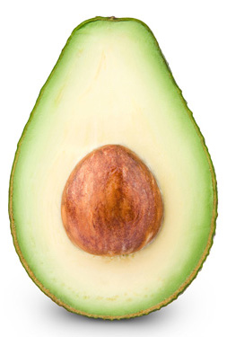
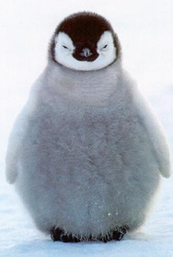
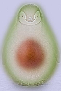
Avocado, Penguin-chick, Avocado Penguin
Frequency Domain Analysis
These are the frequency domains of input images einstein, marilyn and of output hybrid image
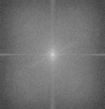
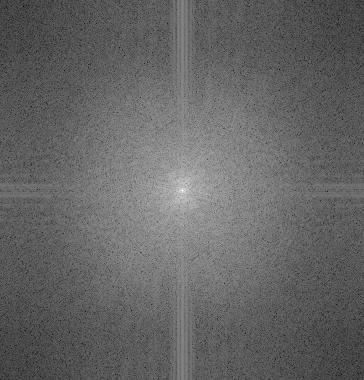
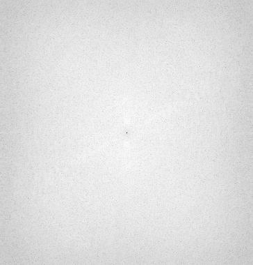
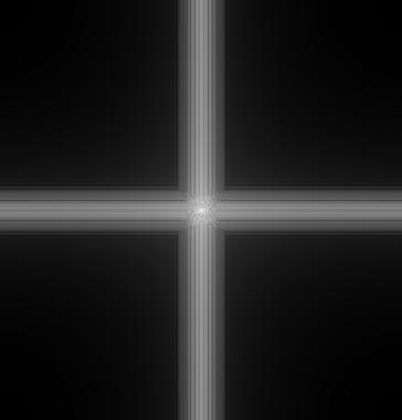
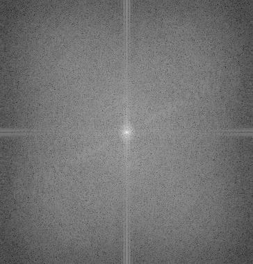
High Freq Input, Low Freq Input, High Freq Input (filtered), Low Freq Input (filtered), Hybrid
Part 1.3: gaussian and Laplacian Stacks
The Gaussian stack was created by recursively applying Gaussian blur to the input image. The Laplacian stack was created by taking the difference between input in layer i and input in layer i-1 in the Gaussian stack.
Scene 1: Example Gaussian and Laplacian Stacks
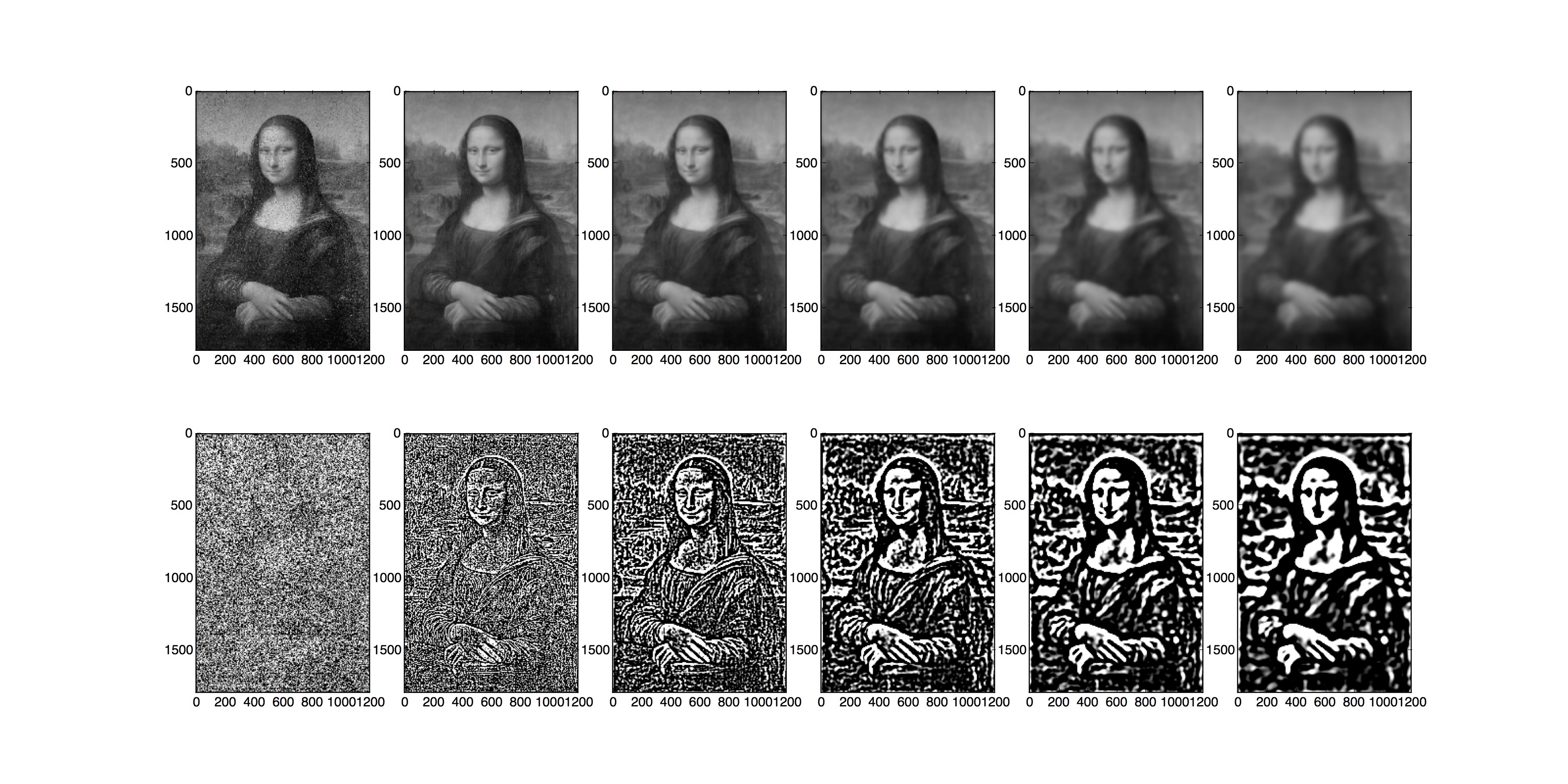
Mona Lisa
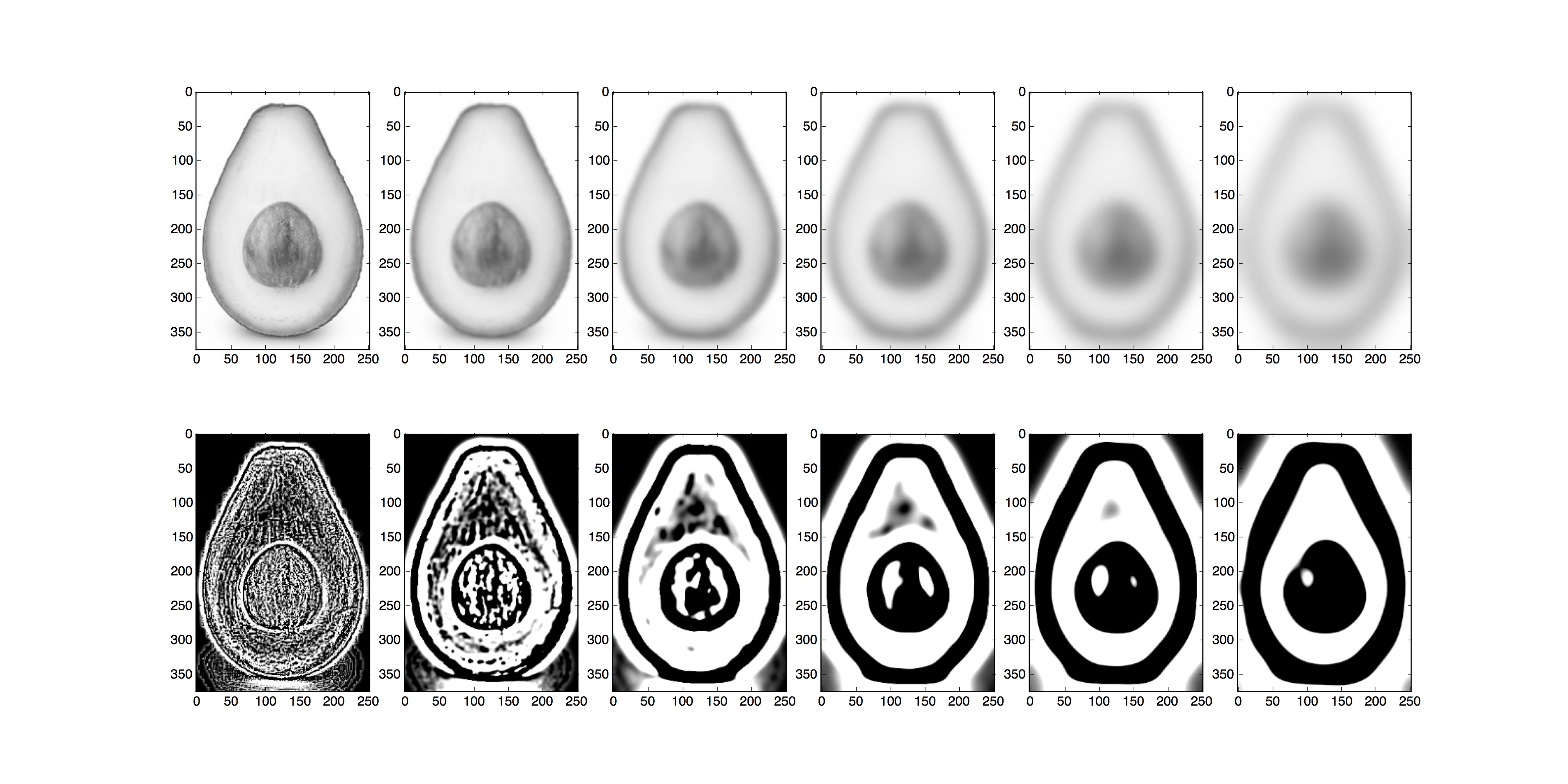
Avocado
Part 1.4: Multires Blending
I used the Gaussian and Laplacian stacks from 1.3 with images f_1, f_2 and mask m. I generated the laplacian stacks, gaussian stacks, and gaussian stacks for f1 and f2, the mask, and the naively blended (concatenated) image.I summed the laplacian stacks with each layer scaled by the mask. I then add this result to the last (blurriest) layer of the gaussian stack from my naively blended image. I noticed that the difficulty was how to use more universal parameters to each image, and how some frequencies were too blurred to show up enough compared to the high frequency components (high frequencies weren't sufficiently masked out enough by the mask gaussian stack).
f_blend = sum_i(gstack_mask[i] * lstack_f1[i] + (1-gstack_mask[i])*lstack_f2[i])
Scene 1: Oraple


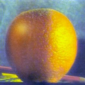
(from left to right) apple, orange, naive oraple, oraple, sigma=1.5
Scene 2: Avotoro
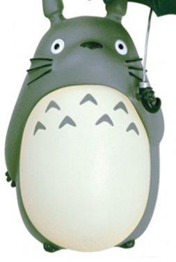
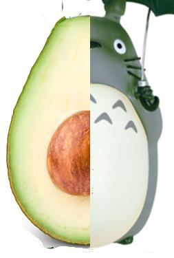
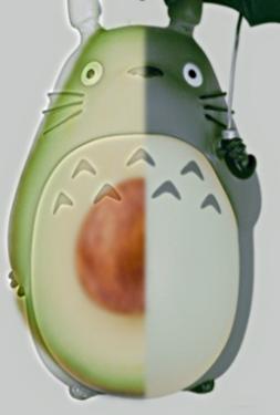
(from left to right) avocado, totoro, naive blend, blend sigma=0.3
Scene 3: Pufferball
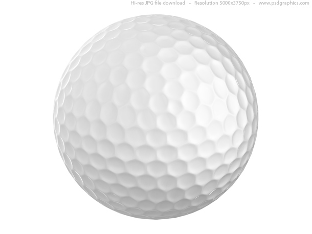
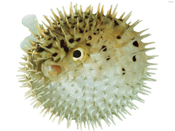
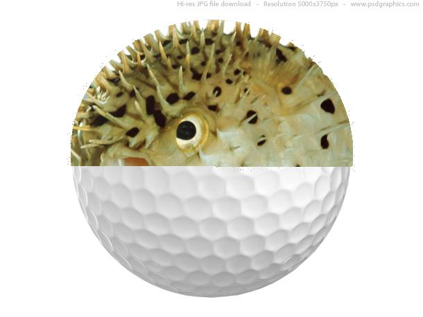
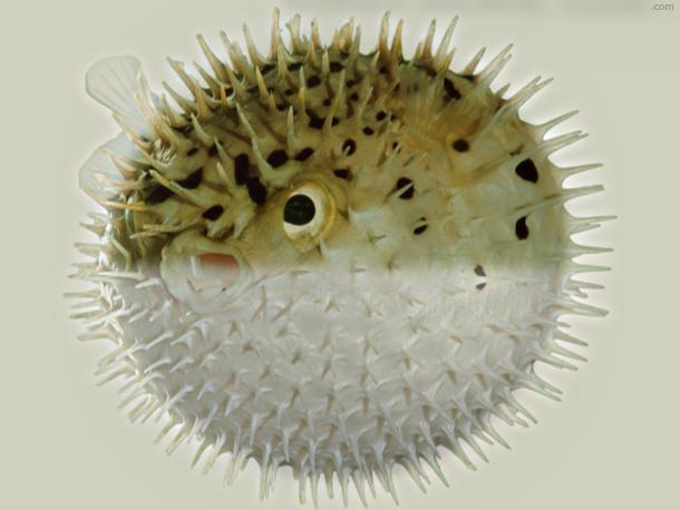
(from left to right) golf, puffer, naive blend, blend sigma=0.6
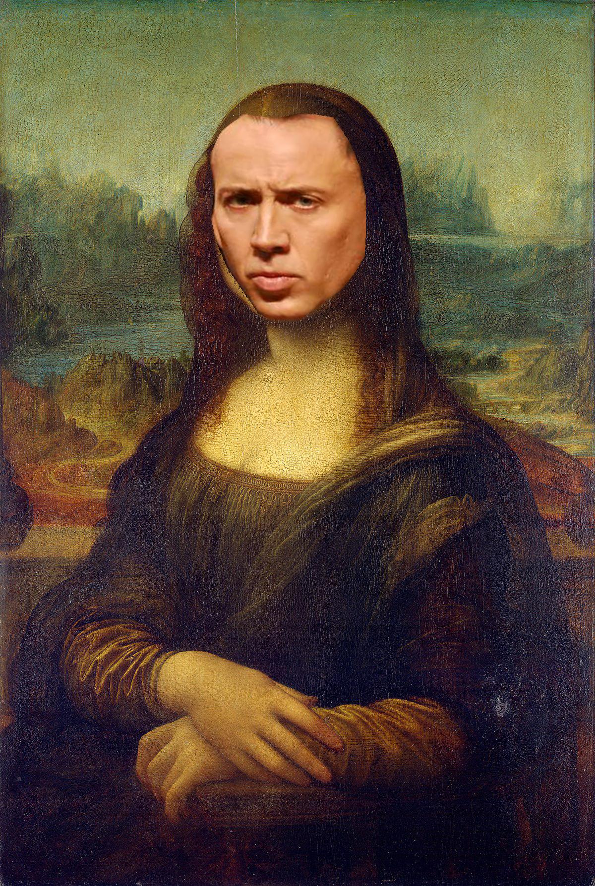
Scene 4: National Treasure
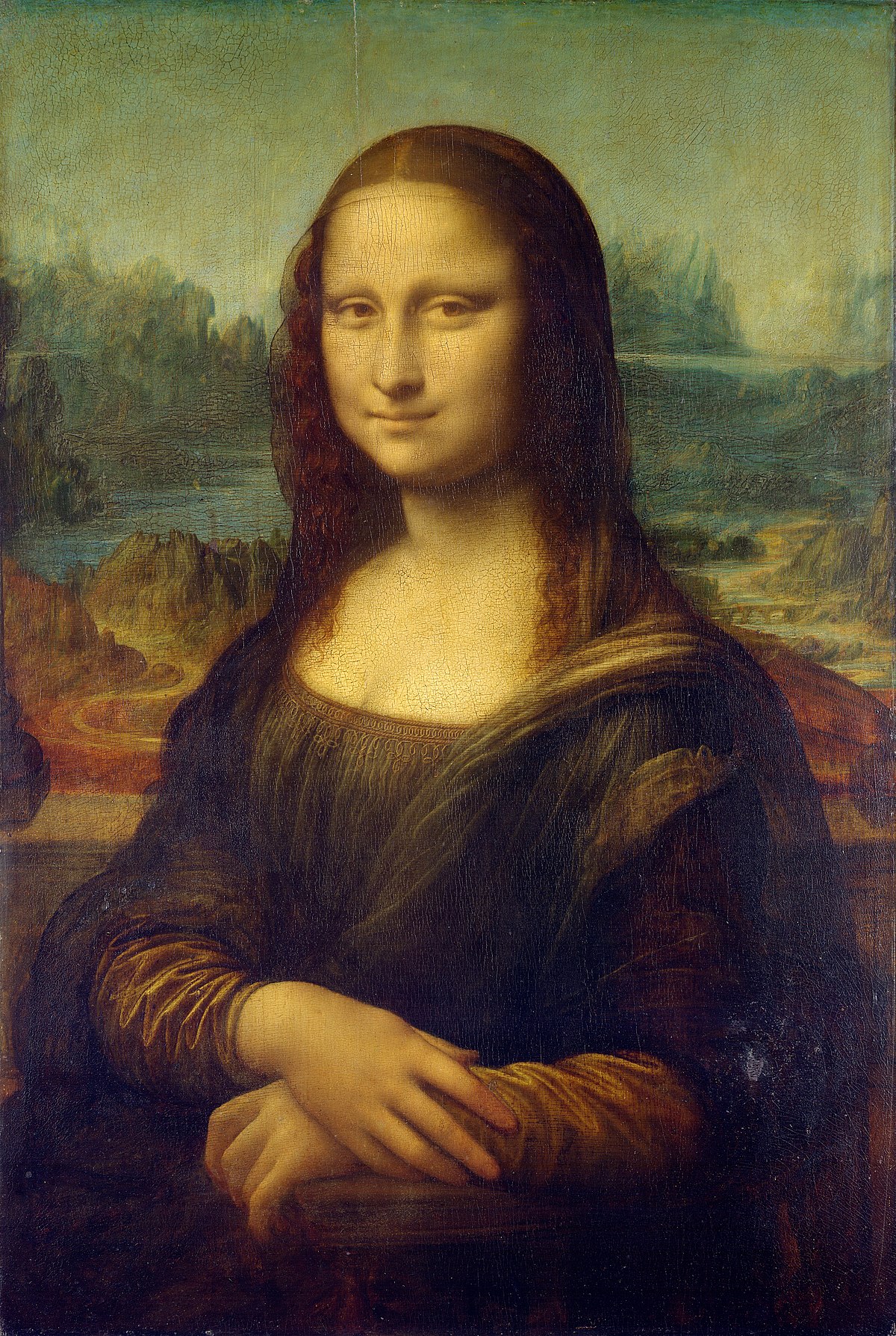
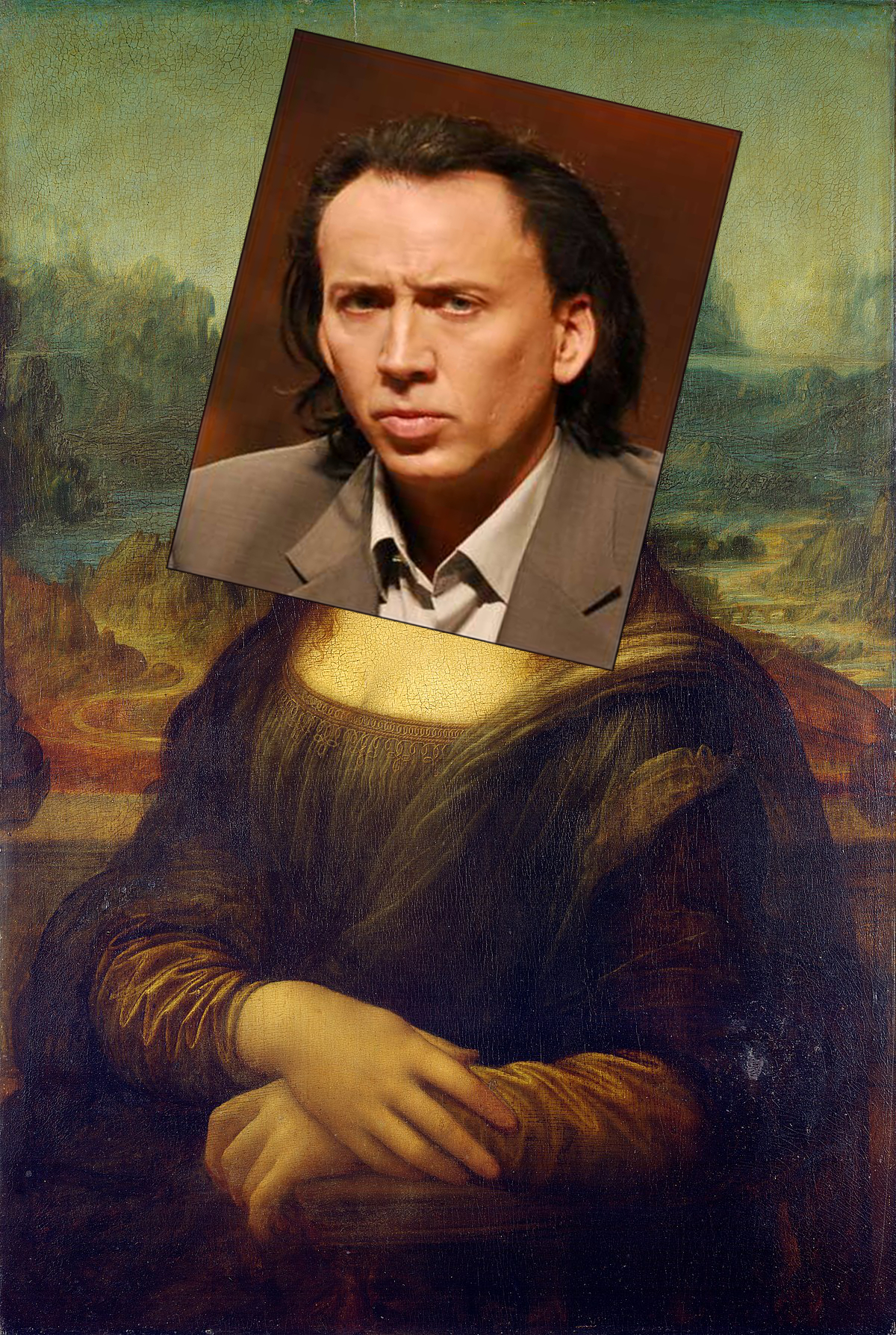
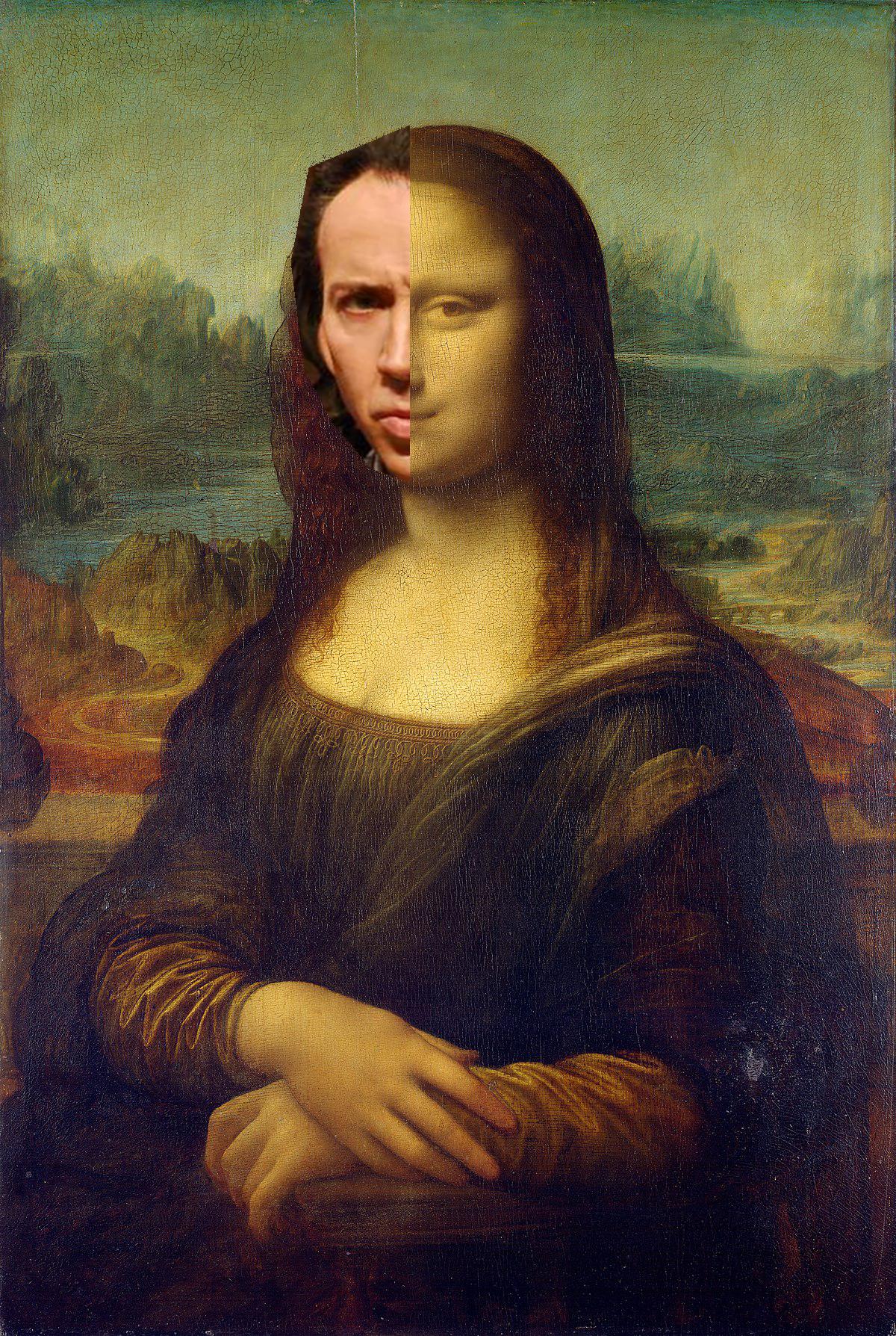
(from left to right) Mona Lisa, Nicolas Cage, naive blend, blend sigma=0.6
Gaussian and Laplacian Stacks
These are the frequency domains of input images einstein, marilyn and of output hybrid image
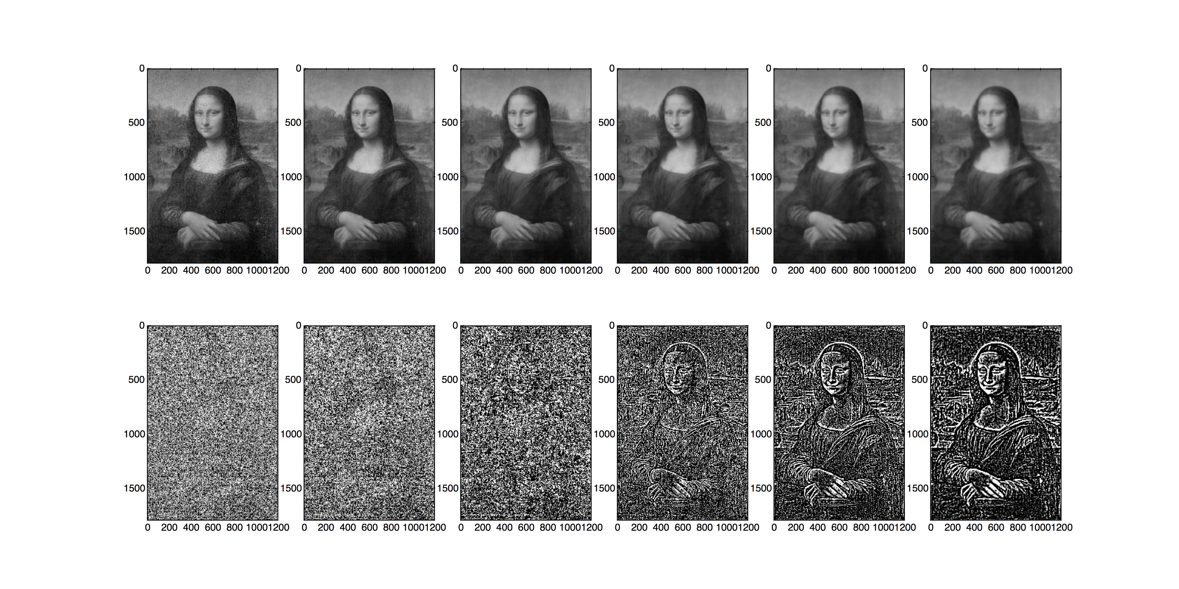
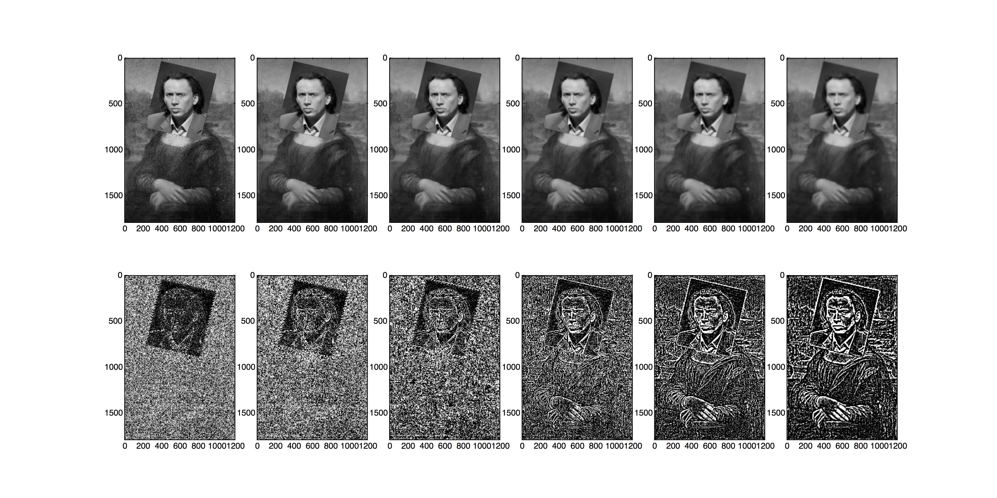
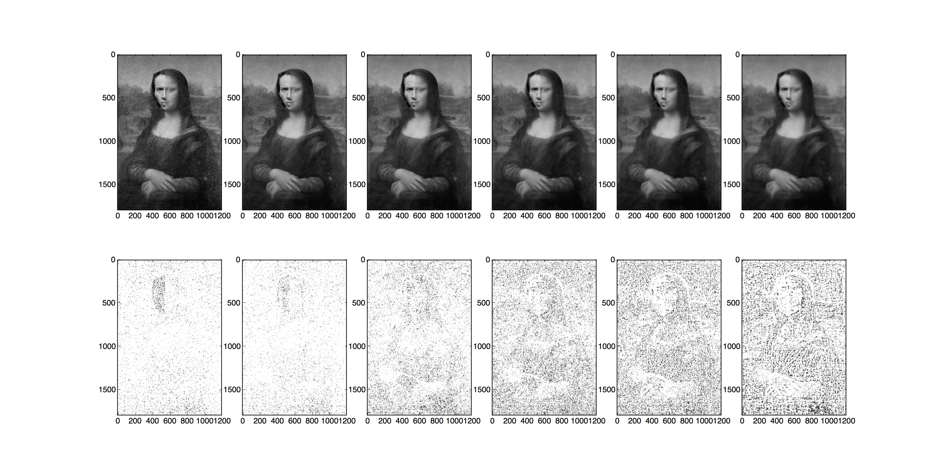
(Top: Gaussian, Bottom: Laplacian) Mona Lisa stacks, Nicolas stacks, Blended stacks
Part 2: Gradient Domain Fusion
Gradient domain fusion is another way to combine images by maintaining their gradients. Set up a least squares minimization problem, Ax = b, where x is the pixel variables you're solving for, b = objective gradient values with the constraint that pixels outside of a mask should be the same value.
Part 2.1: Toy Problem
Set up a linear system Av = b. A is sparse with dimensions (2*h*w+1, h*w). Let v = variable([x, y]), which is the unraveled pixel index. The top half of A represents horizontal gradients of image f: A[v, v] = f[x, y] - f[x, y+1]. The bottom half of A represents the vertical gradients of image f: A[2*v, v] = f[x, y] - f[x+1, y]. The very last row should enforce output[0,0] = source_img[0,0] pixel values: A[2*h*w, 0] = source_img[0,0]
Scene 1: Turtle

original, recovered; L2 error = 0.0625419229608
Part 2: Gradient Domain Fusion
Gradient domain fusion is another way to combine images by maintaining their gradients. Set up a least squares minimization problem, Ax = b, where x is the pixel variables you're solving for, b = objective gradient values with the constraint that pixels outside of a mask should be the same value.
Part 2.1: Toy Problem
Set up a linear system Av = b. A is sparse with dimensions (2*h*w+1, h*w). Let v = variable([x, y]), which is the unraveled pixel index. The top half of A represents horizontal gradients of image f: A[v, v] = f[x, y] - f[x, y+1]. The bottom half of A represents the vertical gradients of image f: A[2*v, v] = f[x, y] - f[x+1, y]. The very last row should enforce output[0,0] = source_img[0,0] pixel values: A[2*h*w, 0] = source_img[0,0]
Scene 1: Turtle
original, recovered; L2 error = 0.0625419229608
Part 2.2: Poisson Blending
We use a variation of the Laplacian to define our gradients: delta = [[0, -1, 0], [0, 4, 0], [0, -1, 0]]
We try to satisfy the following equation. Given the pixel values of source s and target t, we solve a least squares equation for pixel values v, where v represents the pixels from np.ravel(v_img) where v_img is the output image. Each i is a pixel in source region S, and each j is a NSEW neighbor of i. The first summation constrains gradient values to match gradient values inside the mask. The second summation constrain gradient values to match that of the target image for pixels along the mask's boundary.

Source images that had different textures or have brighter regions than the neighboring target pixels would perform worse because the boundary gradients won't necessarily satisfy the interior gradients (would just end up as a blurry image of the exterior), because the solver would gravitate towards solving for brighter pixel values (since we don't have regularization), and/or because the source object was near a strong edge. I used pyamg (Algebria Multigrid Solvers for python) to solve for multiple lstq problems simulataneously. https://github.com/pyamg/pyamg
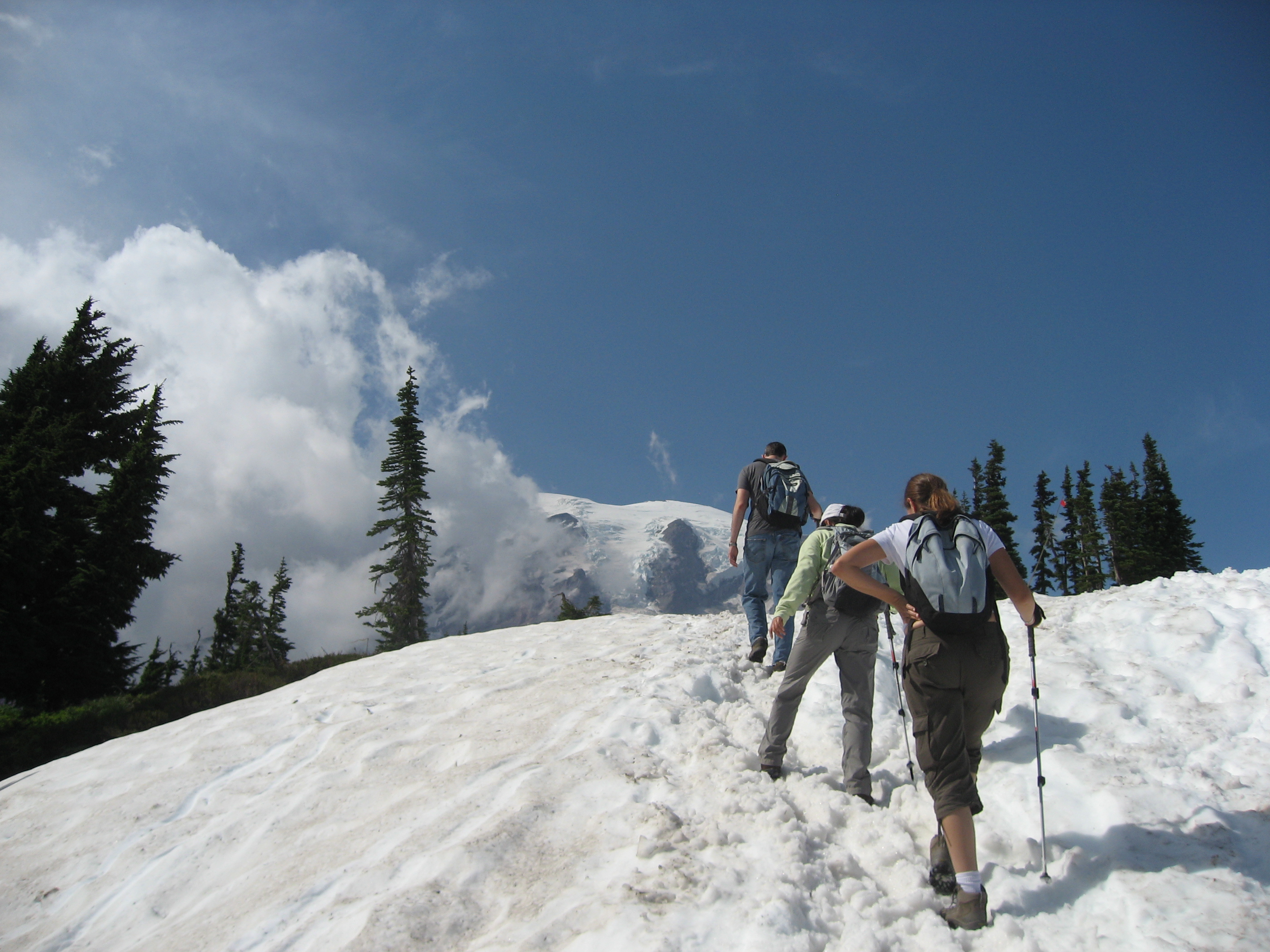
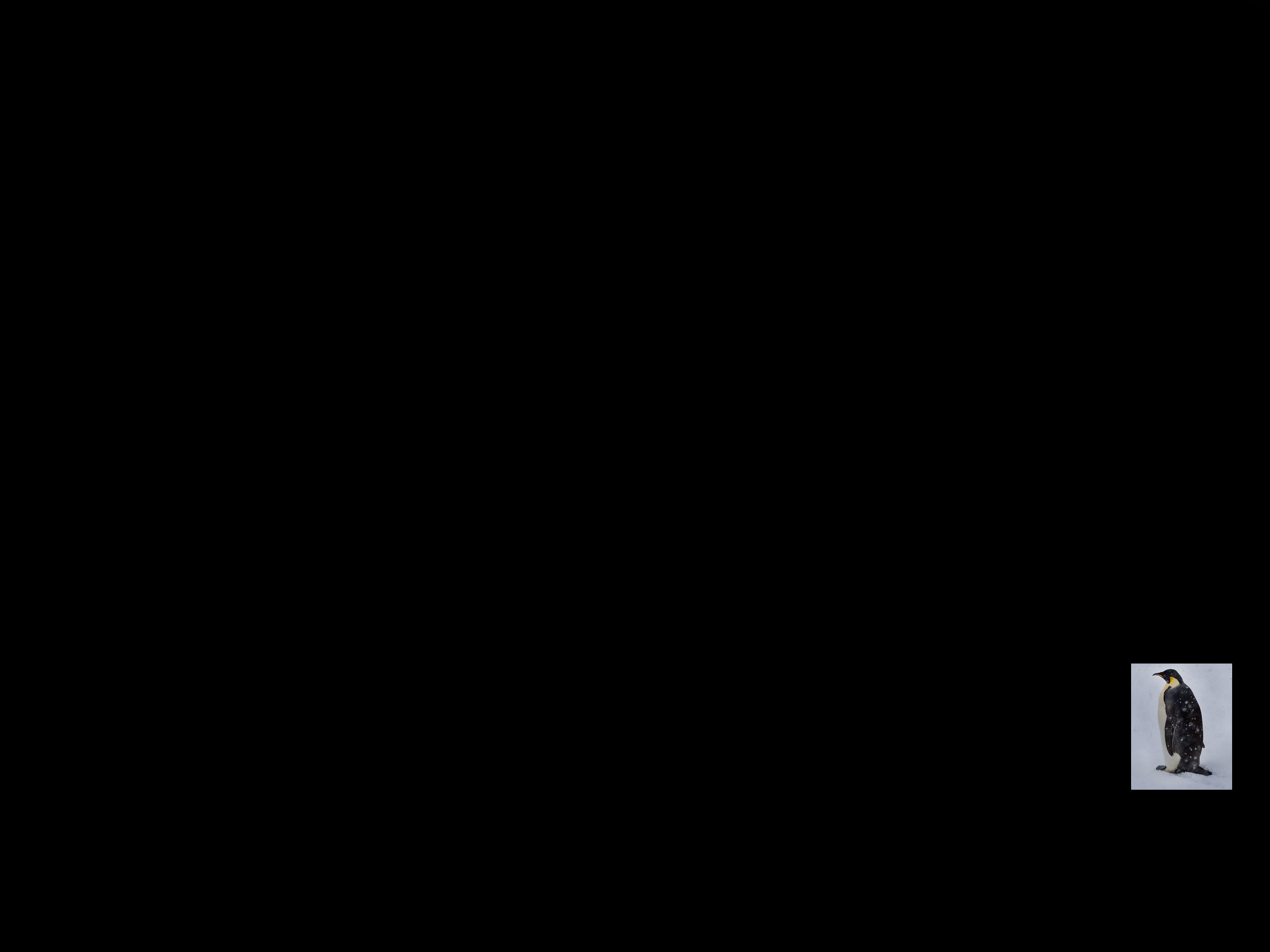
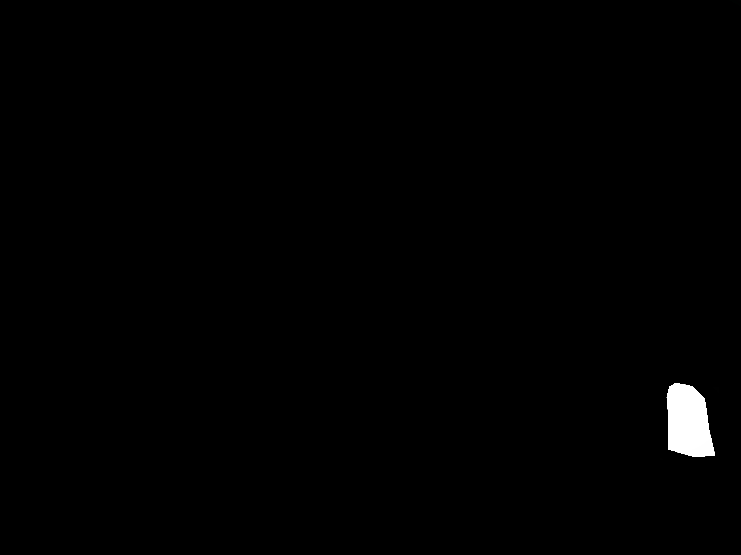
Scene 1: Penguin People
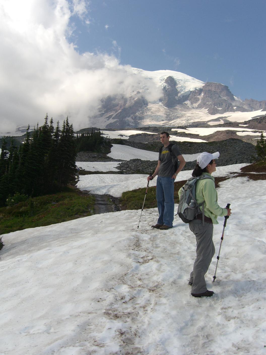
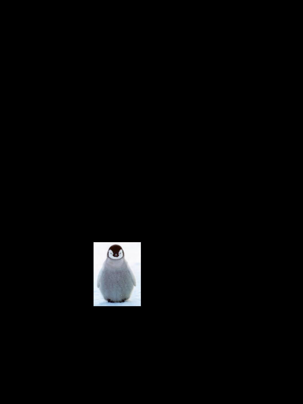
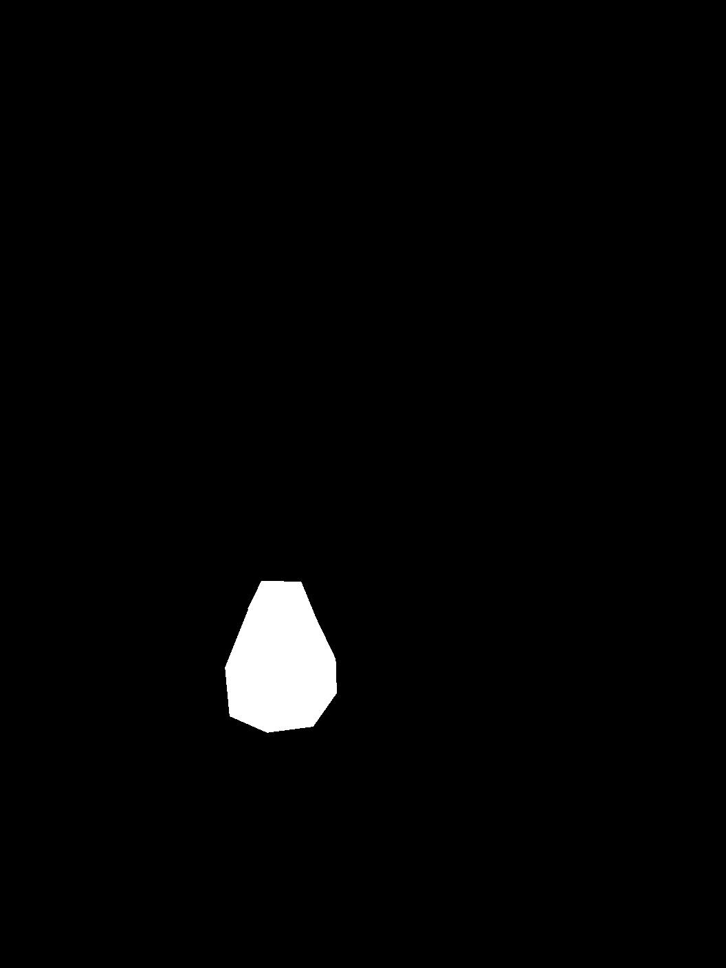
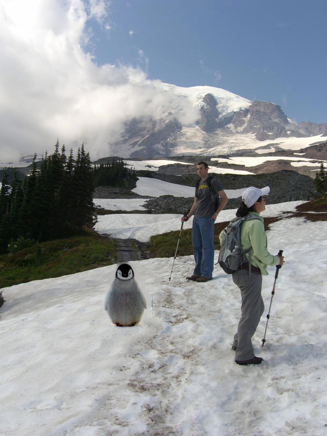
target, source, mask, prediction
Scene 2: More Penguin People (failed)

target, source, mask, prediction
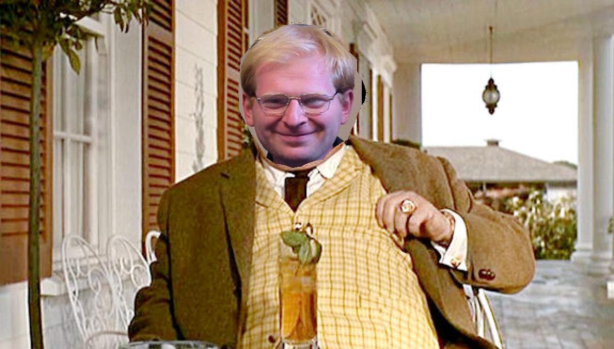
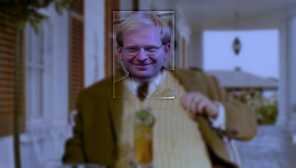
Scene 3: National Treasure

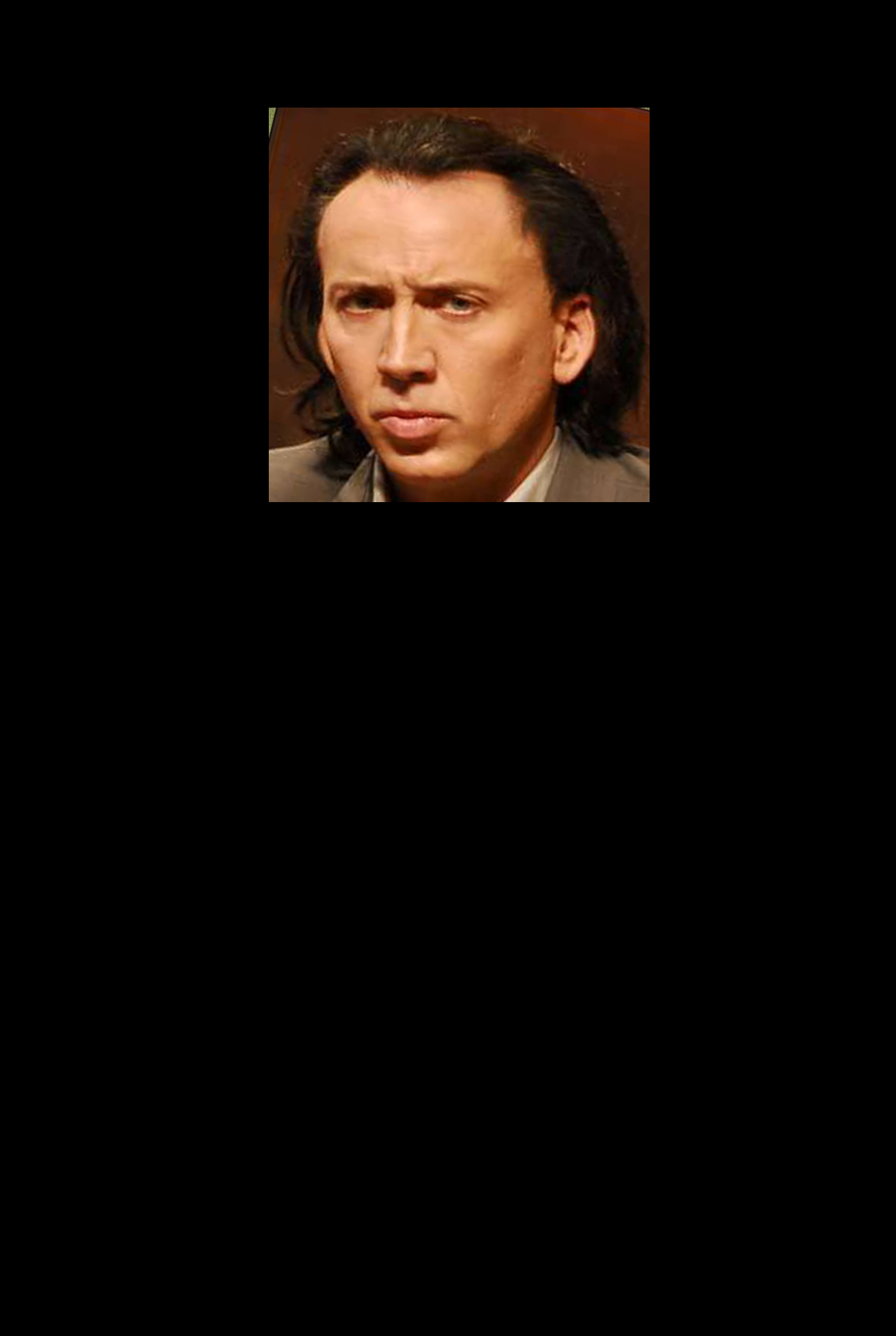
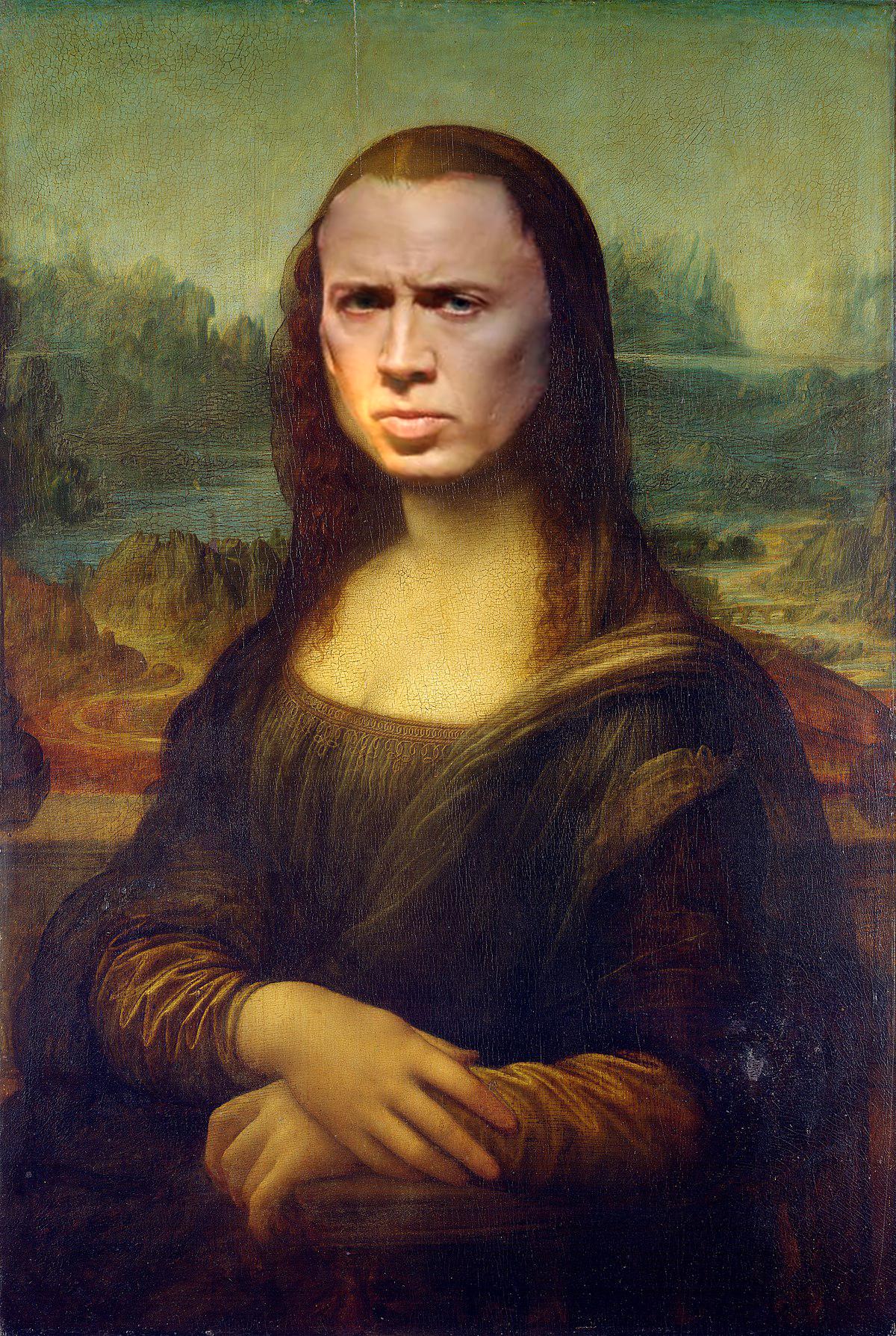
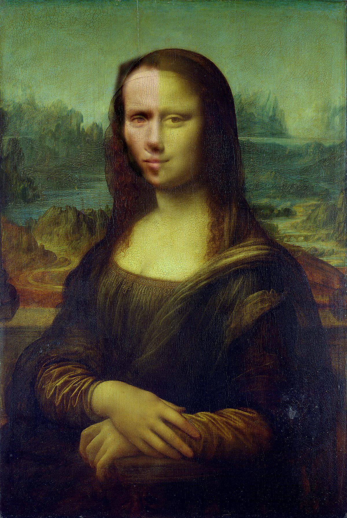
target (mona lisa), source (nicolas cage), source mask, prediction
Scene 3: Goldtography (failed)
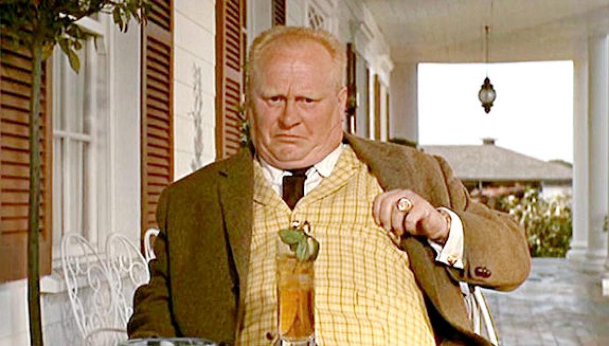
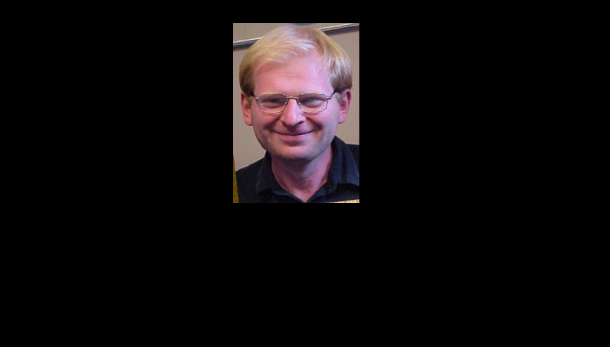
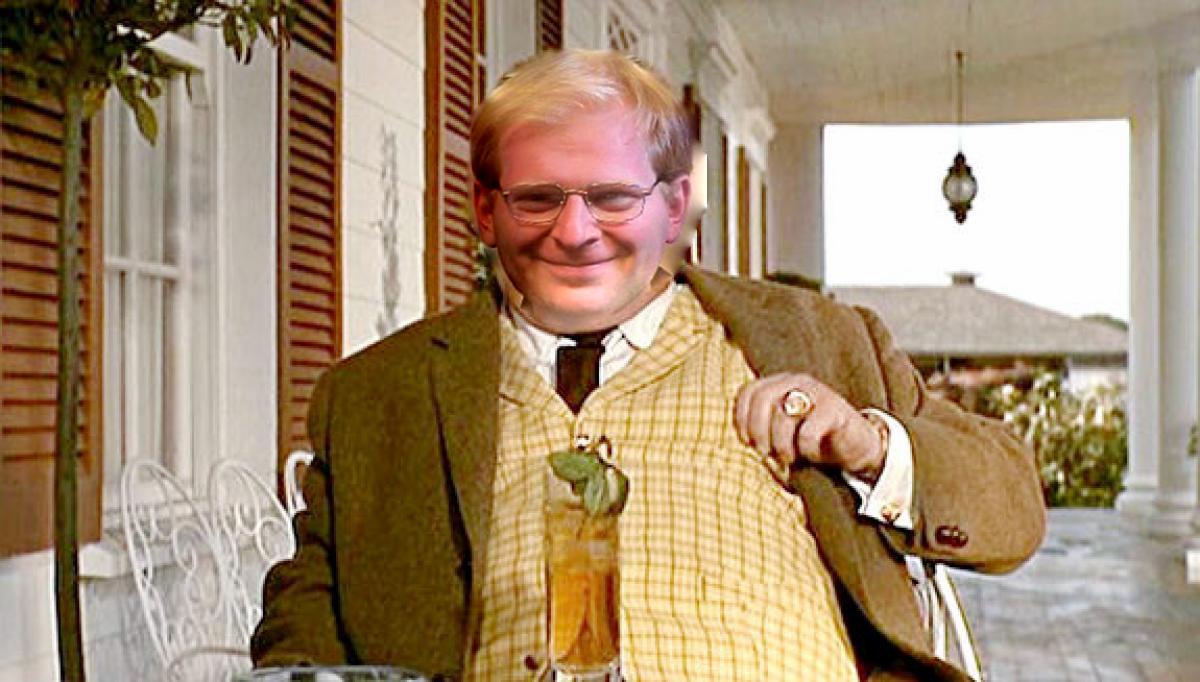
target (goldfinger), source (efros), source mask, prediction
Blending techniques comparison
The poisson output looks smoother, especially since it was concerned with maintaining gradients. The multires blending technique keeps the original hues of each image a bit more (more concerned with how close the colors are to the original images).
Scene 1: National Treasure
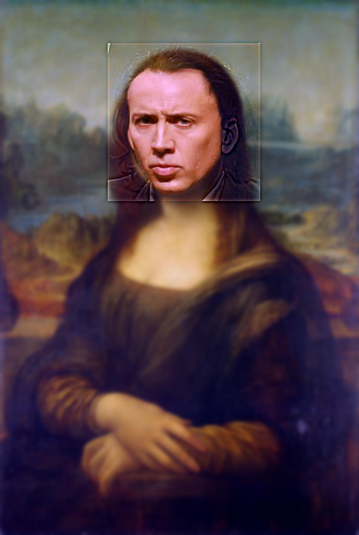
naive, multires blend, poisson blend
Scene 2: No Mr. Bond, I expect you to die.
naive, multires blend, poisson blend
Reflection
This project showed me the pros and cons of different implementations of the same concept (manually setting gradients vs convolving with a laplacian, or cv2.GaussianBlur vs scipy.ndimage.gaussian_filter, or scipy.sparse.linalg.lsqr vs pyamg.solve). I learned to actively use popular image processing libraries such as opencv and scipy.