Overview

There are many ways to blend images together. You could go into Photoshop right now and average pixel values together, adjust the transparency of the images, carefully erase overlapping boundaries by hand, etc. But these different approaches still all exist in the spacial domain. This project is an exploration into manipulating images in different domains by taking advantange of mathematical or structural properties. Part 1 explores the frequency domain, making use of high-, low-, and band-pass filtering. Part 2 examines how image gradients can be used to create ever more powerful blending effects.

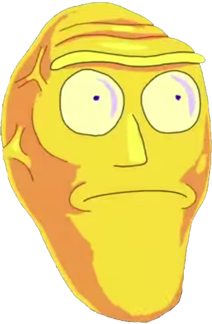
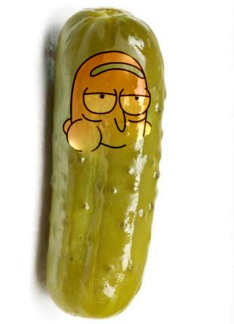
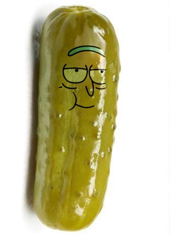
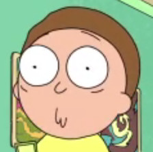
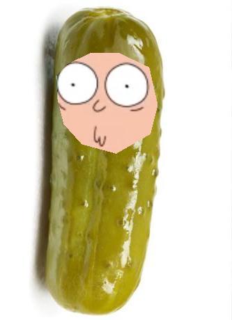
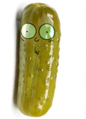
If you're a Rick & Morty fan, you'll love Part 2.

Part 1: Fun with Frequencies!

1.1 - Warmup: Image Sharpening

We usually think of an image as a grid of pixels, but it can also be represented as a collection of signals across different frequencies. Fine details are carried through higher frequencies, and low frequencies resemble blurrier, more general patches of information. Knowing this, we can manually sharpen an image by extracting the high frequencies from an image, and boosting them in the original image. There are 2 ways to do this:
1. Blur the image by convolving with a low-pass filter and take the difference betwee this and the original image. Then add back these extracted details scaled by a parameter α
2. By the results below, the order of operations can be rearranged so that a single "sharpening" filter is created that is then convolved directly with the original image to get the same effect. This approach is called "unsharp mask filtering"

f +α(f − f ∗g)=(1+α)f −α f ∗g = f ∗((1+α)e−αg)

These results were created with α=1.5, σ=2

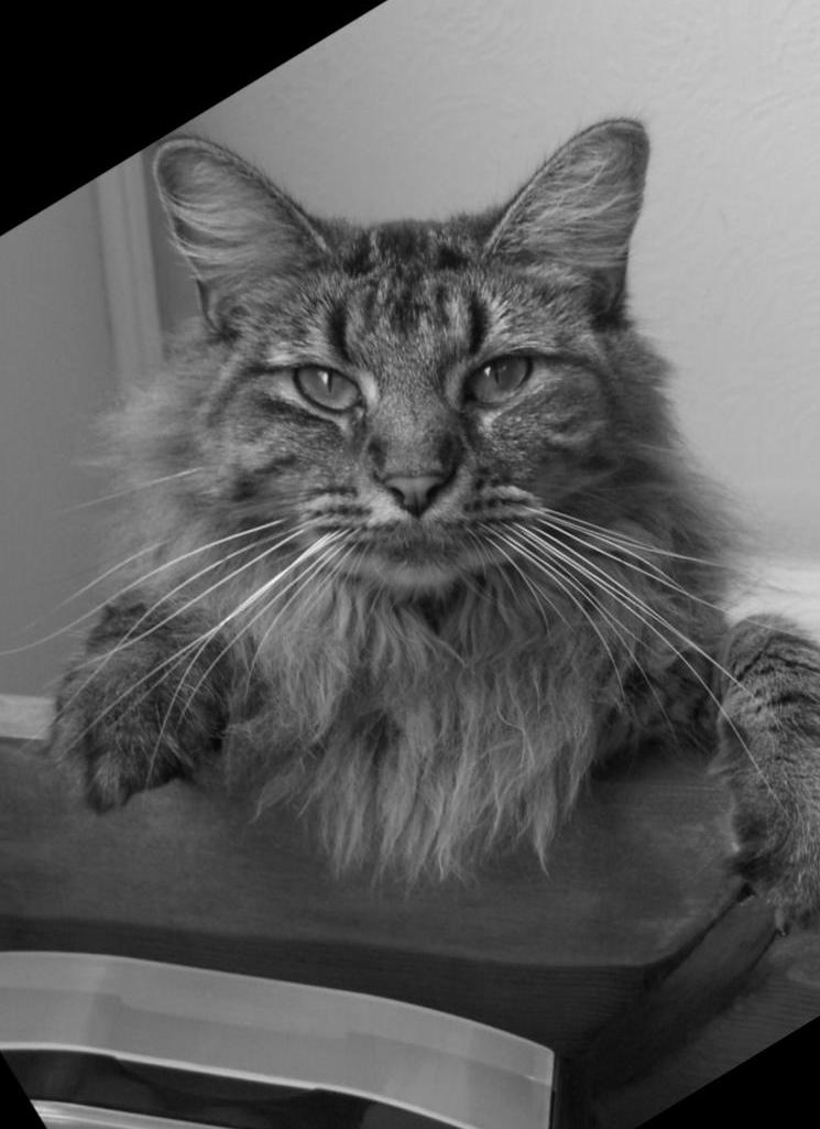
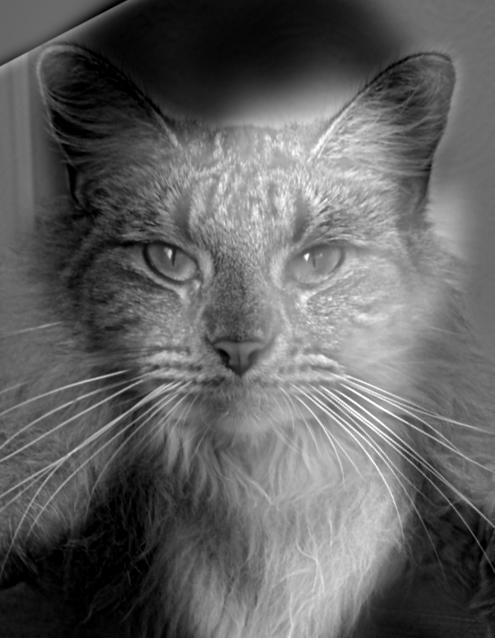
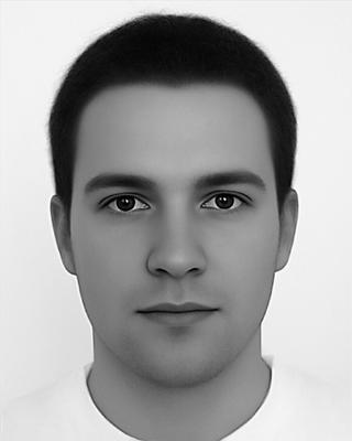
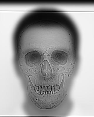
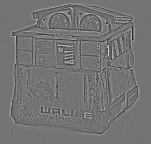
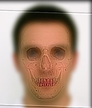
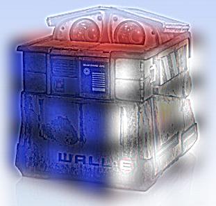
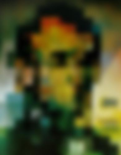
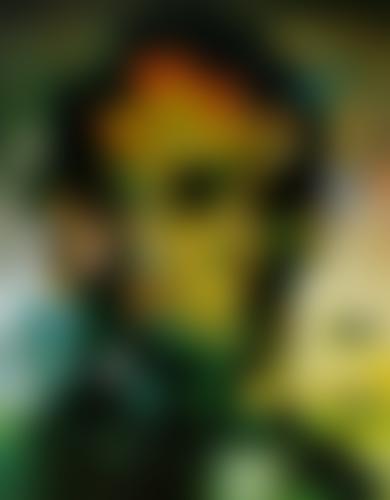
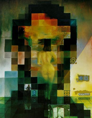
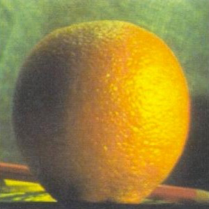
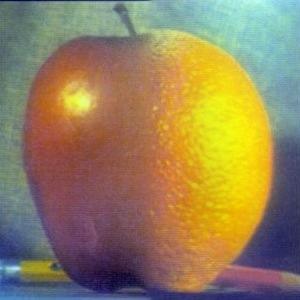
1.2 - Hybrid Images

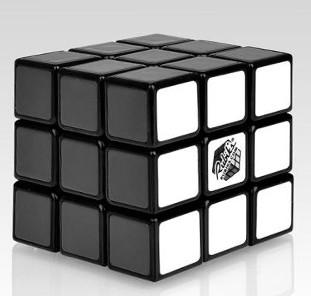
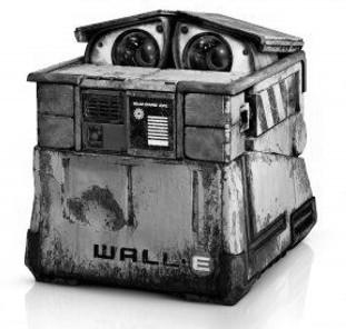
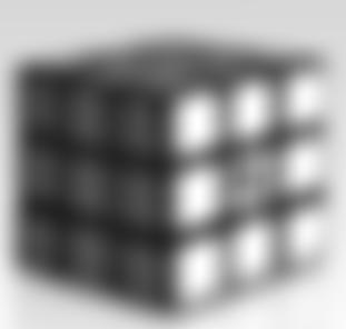
Typically, a single image is composed of frequencies all across a spectrum. But if we process 2 completely different images to occupy separate frequency spaces, they can occupy the same space. Filtering an image with an estimate of a 2D Gaussian is known as a "low-pass filter", as it removes all the high frequencies above a certain cutoff frequency specified when creating the filter. Using the first sharpening technique, we can extract only the high frequencies from the other image using a different cutoff frequency. The result is such that one image (the high frequency one) is visible up close, but if you step a few feet away from the computer you will see the image onscreen mysteriuosly change.

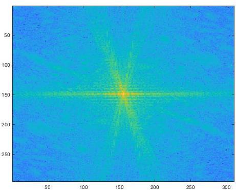
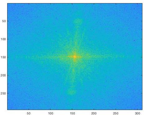
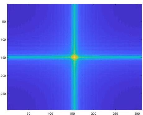
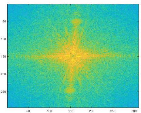
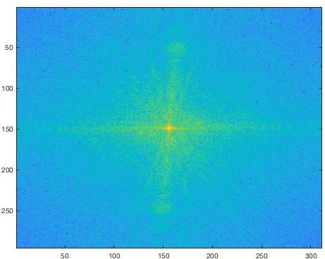
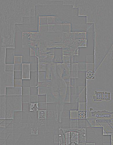
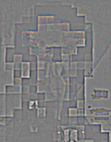
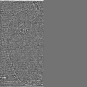
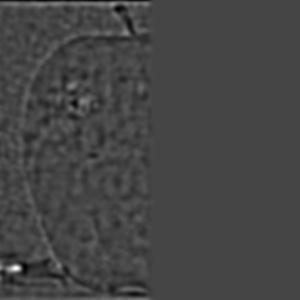
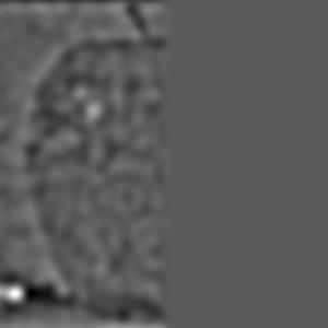
Frequency Analysis

By transforming the images into the frequency through with a Fourier transform we can "see" the high and low frequencies that are being extracted to create the final hybrid image. This is especially visible in the FFT of the low-passed Rubik's cube.

☆ Bells and Whistles

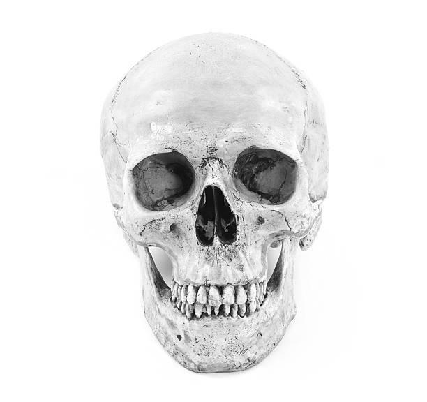
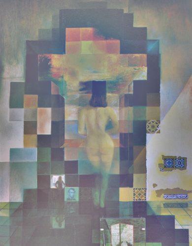
For the main hybrid image results I grayscaled the input images before overlaying them. I then tried the results by leaving color in one or both of the inputs. The results were mixed – in the skull image pinkish color of the face in the background somewhat matches the hue of aged bone, and so the look feels natural. Either way, I found that leaving the background colored had a greater effect if any.

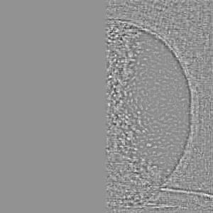
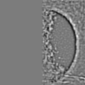
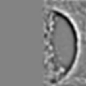
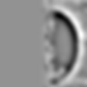
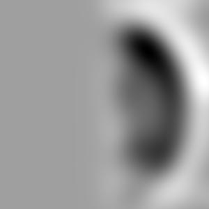
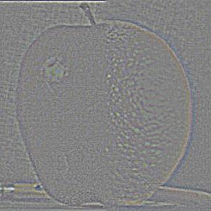
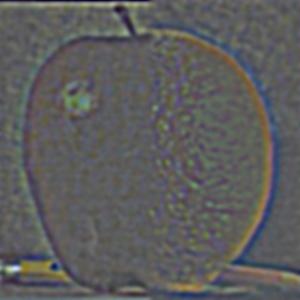
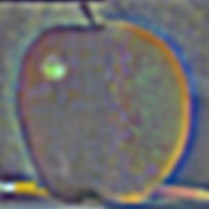
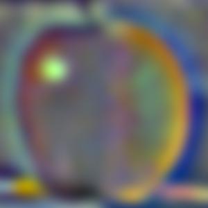
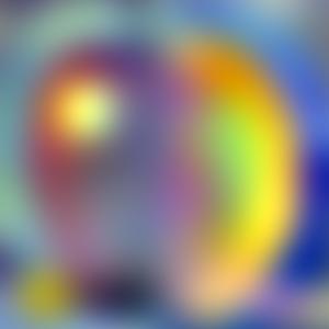
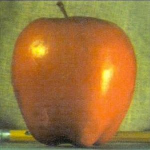
1.3 - Gaussian & Laplacian Stacks

A Laplacian stack breaks up an image into frequency bands, where each image in the stack (2nd row) contains only the frequencies in the image that lie in a certain range. This project used a typical range of powers of 2, known as octaves. Each frequency band is just the difference between 2 layers of a similar Gaussian stack and the same as the sharpening effect from 1.1.

Interestingly, we can reconstruct the original image from this stack of high frequencies by simply summing them up – almost. Since each Laplacian stack layer is the result of the difference between 2 Gaussian filtered stack layers, summing up just the high frequencies gives us the result on the bottom left. This stack was created with N = 5 layers, but this means that a 6th Gaussian layer was created. Adding this lowest Gaussian layer to the sum of the Laplacians gives us the original image on the right.

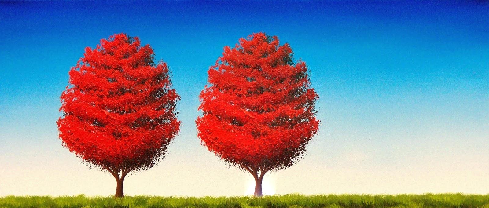
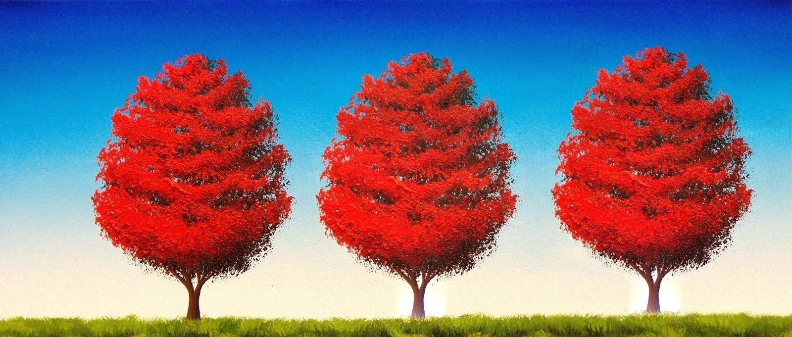
1.4 - Multiresolution Blending

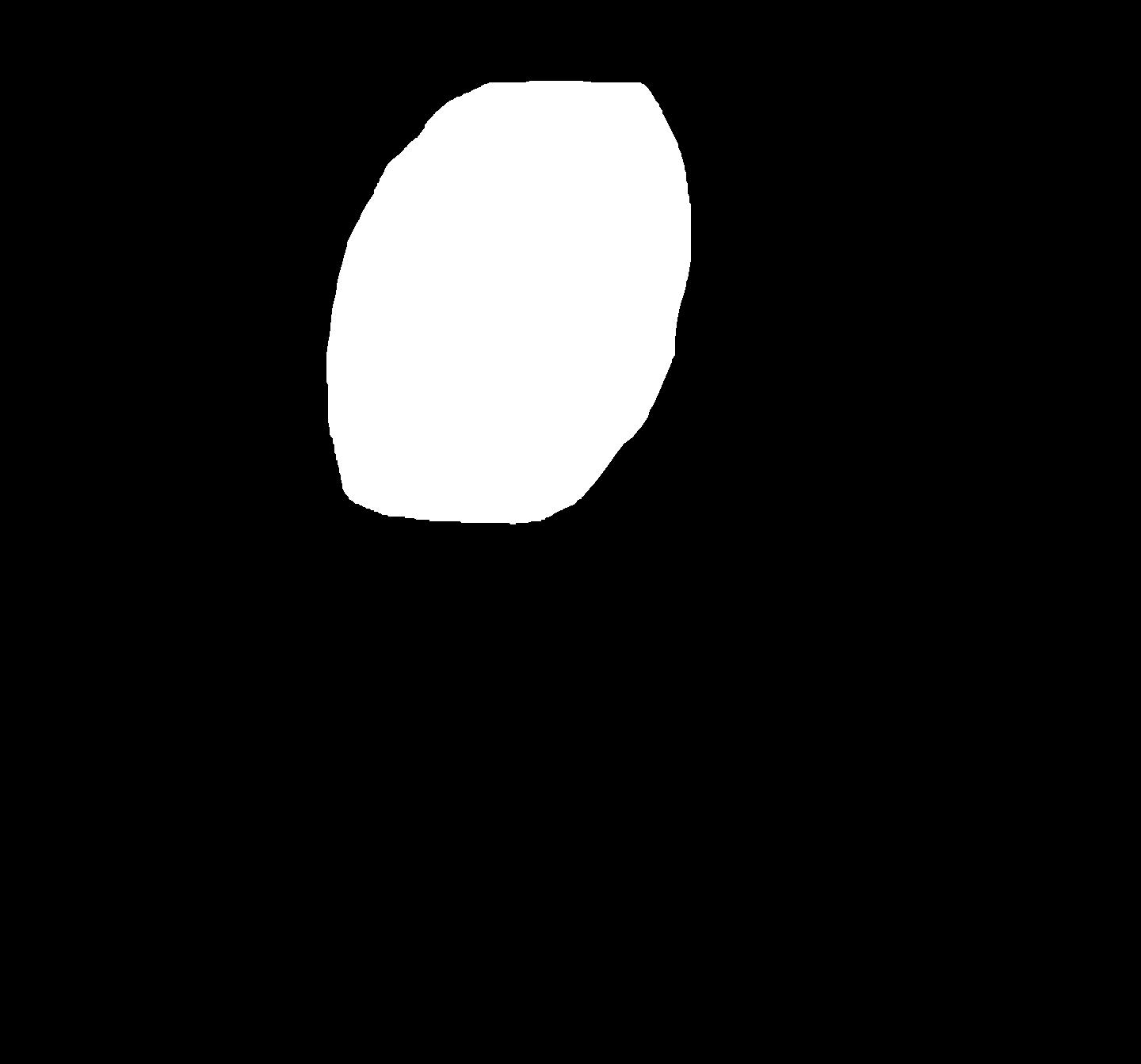
Given a binary mask, 2 images can be blended together by feathering the edge of the mask, multiplying each image by the mask or its complement, and summing them together. But some frequencies along this boundary may average together well, while others may not. Multiresolution blending solves this by breaking the 2 images down into frequency bands and blending them separately at each level. This gives much better results, which can be improved even further by blending separately in each color channel. A Gaussian stack is also produced for the mask itself to blend at each layer of the stack.

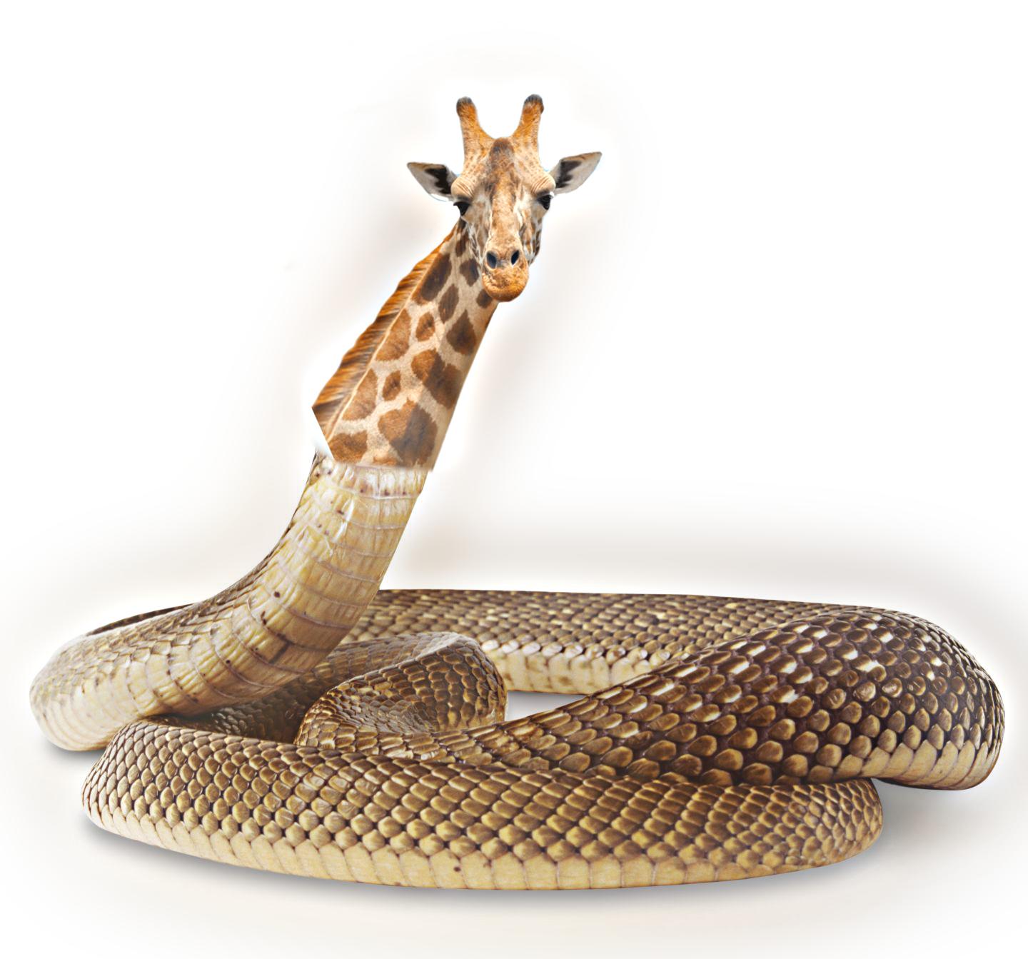
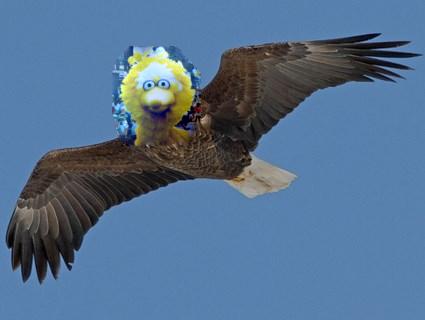
Hybrid Animals

Part 2: Gradient Domain Fusion

2.1 - Warmup: Image Reconstruction

Now we are back in the gradient domain, where our images are thought of as 2D grids of intensity values, usually in 3 color channels. This grid structure allows us to calculate discrete gradients; in the y direction, we can calculate (x,y+1)-(x,y) for every pair of neighboring pixels. This representation be extended to the entire imgae to form a system of linear equations, as a 2D image can easily be flattened into a 1D vector.
This warmup exercise does exactly that: given an input image, a linear system is set to create a new output image v that matches the x and y gradients of the input image, as well as the grayscale intensity. Each pair of pixels forms an equation for each gradient direction, trying to match the gradients in the same spot in the original image. After solving this system contains pixel values that match the original image almost exactly.

2.2 - Poisson Blending

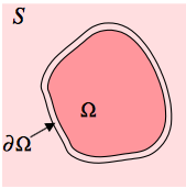
A paper by Perez et al. 2003 intoduced the concept of blending images via their gradients, which they called Poisson blending. The minimization problem is listed below, but the picture to the right also helps to visualize the relationships to consider. To blend an arbitrary area of a source image into a target image (the target is confusingly called "S") the user defines an area Ω. To represent this mathematically we want a vector v representing the pixels of the output image that minimizes the difference between the source and target gradients. The 2 separate terms introduce the boundary conditions which are represented by ∂Ω in the diagram. Essentially for each pixel of the source image inside the area Ω, any neighbor pixels that are on not inside Ω are assigned to the corresponding intensity from the target image, while neighbors also inside Ω must be determined by the minimization and now form an additional constraint.

Examples

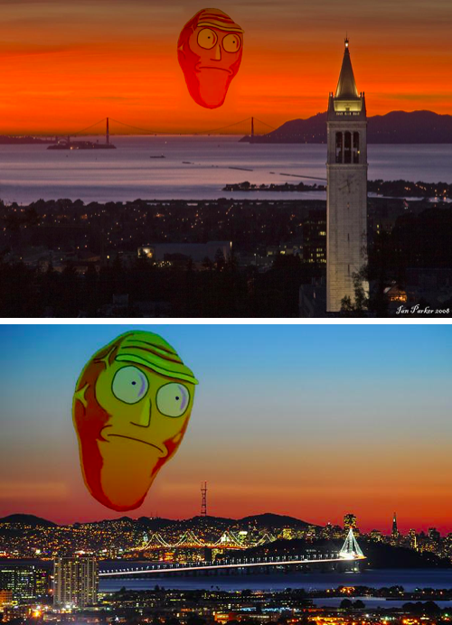
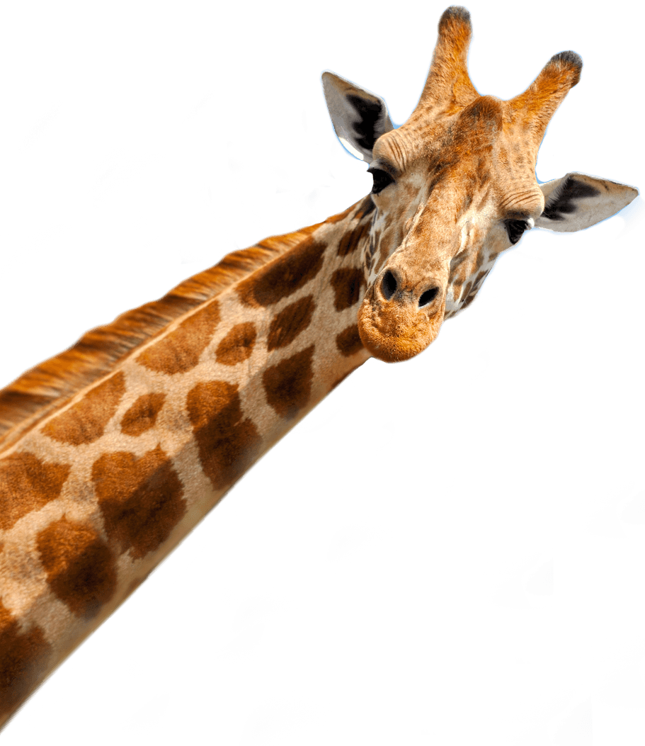
Seamless Cloning

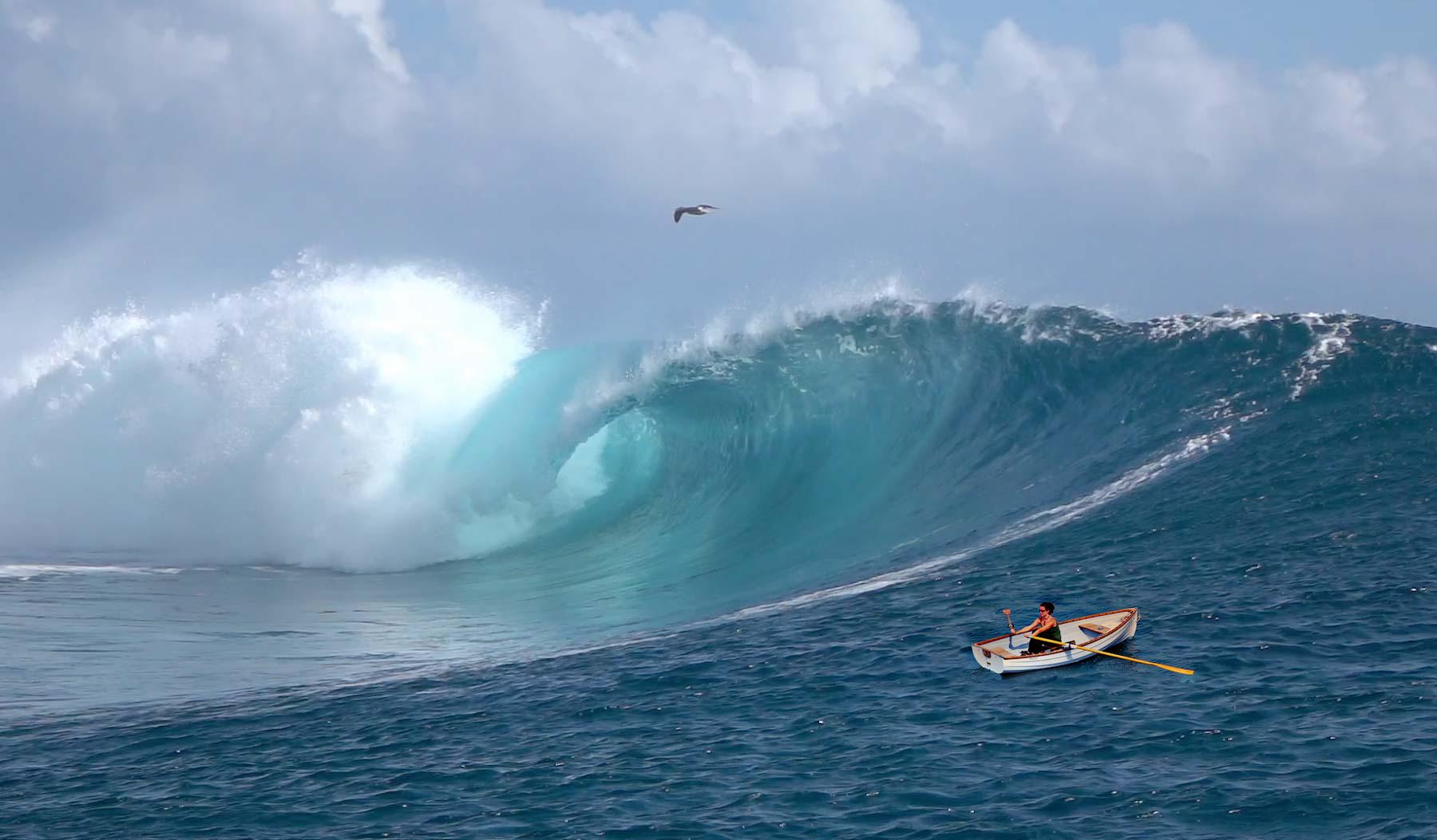
After using the gradient-based method to blend different images together, I decided to experiment with using the same image as both the source and the target (background) image, allowing me to clone objects of interest. Other than specifying a different source image, I used the same workflow to align the images and generate a mask, which is why I think the results turned out so well!

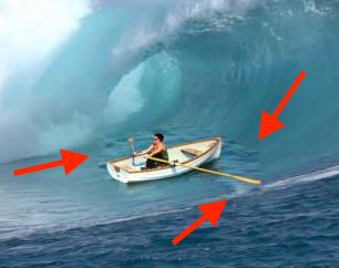
Problems and Failures

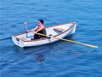
Usually If the area surrounding the object of interest in the source image was fairly simple, or matched the target area nicely, then the process of cutting out the object and generating a mask was allowed to be pretty liberal, as was the case with the penguin and the rowboat respectively. In some of the cases below these conditions weren't met – and the least squares solution had to disrupt the colors of the original image, wasn't able to blend enough, or both in the worst case.

⚡️ Note on Optimization

I exploited some structure of the way the gradients were calculate and used no `for` loops, only vectorized MATLAB code. I calculated the row and column indices of all matrix values, then passed these to a sparse matrix constructor which ended up being much faster than pre-allocating a sparse matrix and indexing into it. The toy problem was only meant to run on a specific small image, which explains the very small runtime of 0.069441 seconds. Even for gradient blending, the process ran on all 3 color channels in about 5 seconds for images that were pre-downsized by 1/2, and well under 30 seconds for full input images.

☆ Bells and Whistles

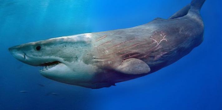
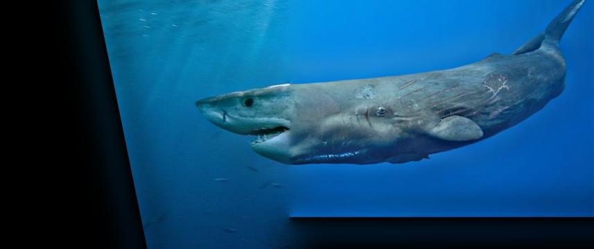
Mixed Gradient Blending

Poisson blending always aims to minimize the error from the target gradient. But if the source image contains very little detail and the background is detail-rich, some areas in the source mask can cause the background to look blurry. Mixed gradient blending fixes this by taking the gradient from either the source or target image with the largest magnitude to compute each pixel-to-pixel neighbor constraint. The new minimization problem is then

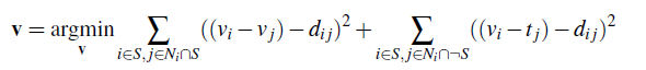
where d_ij = max(abs(s_i - s_j), abs(t_i - t_j))

Comparison of All Methods

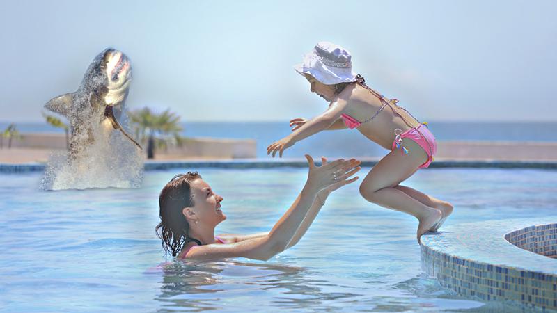
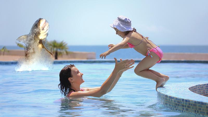
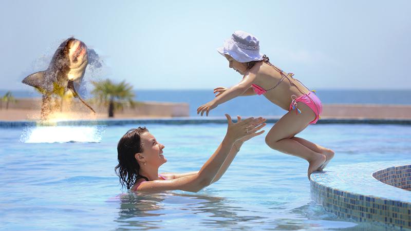
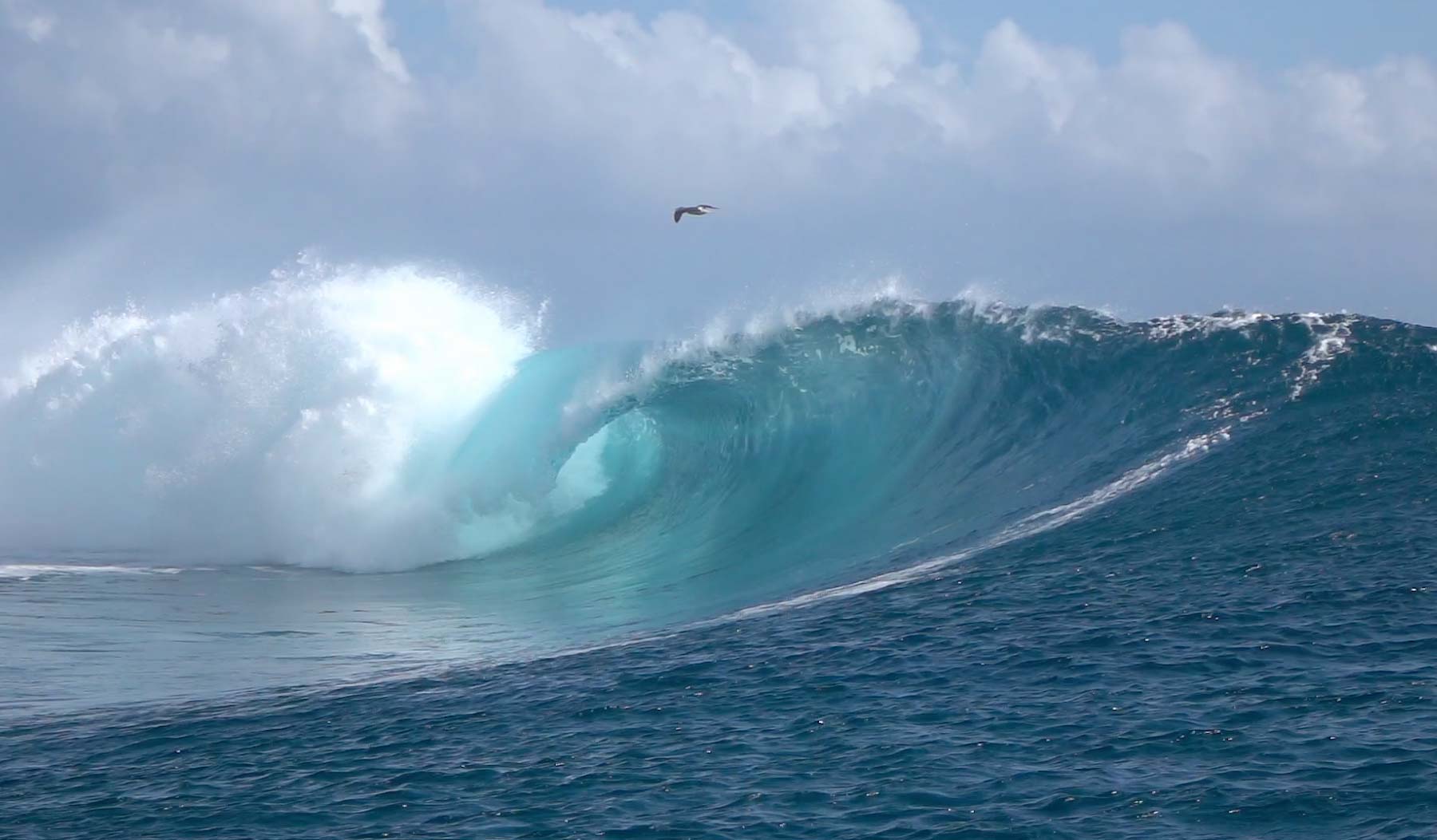
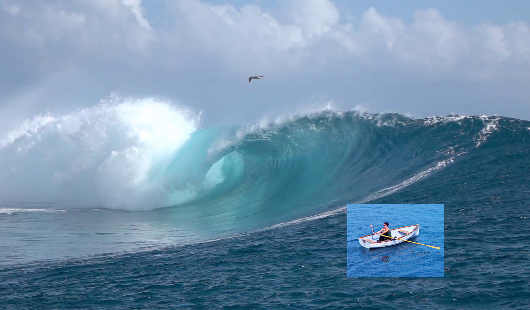
I decided to give the blending algorithms a test with a difficult blend in both images. The shark had lots of water droplets around it, and the area of the background I focused on had some palm trees in the background, which might produce some odd gradients to match. I thought the water at the bottom of both images might've helped the results. I enjoyed working with gradient blending more due to the flexibility with extraneous source pixels inside the mask (even considering the errors discussed earlier). Multiresolution blending is more tedious and requires more effort in creating an accurate mask. Multiresolution blending is also not robust to significant changes in global light patterns, seen above as the shark is too dim compared to the bright outdoor pool. In most cases mixed gradient blending outperformed standard Poisson blending, but I'm glad I found an exception to this. The background colors were just too different, and so the changes to the pasted source colors became drastic. In the end, Poisson blending struck a satisfying middle ground.

Conclusion

This project was a very multi-faceted learning experience for me. Part 1 was my first experience with the frequency domain, filtering, sampling, and much more. Laplacian stacks gave us an avenue to learn how JPG compression works, and learning how to reconstruct images with both frequencies and gradients was intriguing to me. Part 2 was even more impressive because the conceps of gradients and least squares systems was not new to me, but they performed so much better than frequency domain methods that I was still surprised. Setting up matrices with tens of thousands of dimensions for gradient blending really made me appreciate MATLAB's ability to work with sparse systems, as well as a fun refresher in crafting vectorized code.

Thank you for taking the time to view my project, I put a lot of time and heart into making great results because I really enjoyed doing so!