For this part of the project, we had to sharpen an image using the unsharp masking technique introduced in lecture. First I blurred the image using a Gaussian filter with sigma = 10, then subtracted the blurred image from the original image to get the "details" of the image. I then added this back to the original image, resulting in a sharpened image!
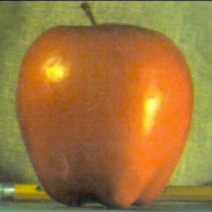
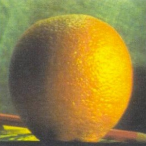
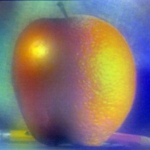
In this part of the project, we blended together two photos, one isolating the high
frequencies and one isolating the low frequencies, so that the blended image would appear
different depending on the distance from which it is viewed from. At a close distance,
the high frequency image should dominate and be visible. At a greater distance, only the low
frequency image should be visible.
To accomplish this, I used a 2D Gaussian filter as a low-pass filter for one image. For the other
image, I used the same low-pass filter, then subtracted the result from the original image to get
only the high frequencies of that image. I experimented with different values of sigma for the
Gaussian filters of each image to determine which value worked best for each image. I used the given
python code to align the images, and then added them to get a hybrid image!
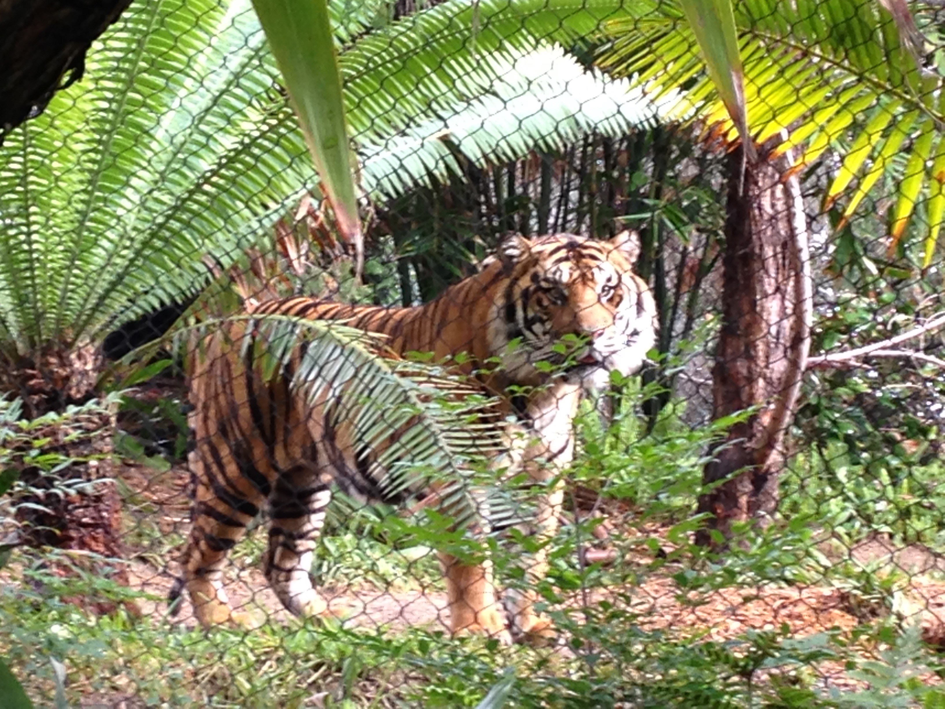
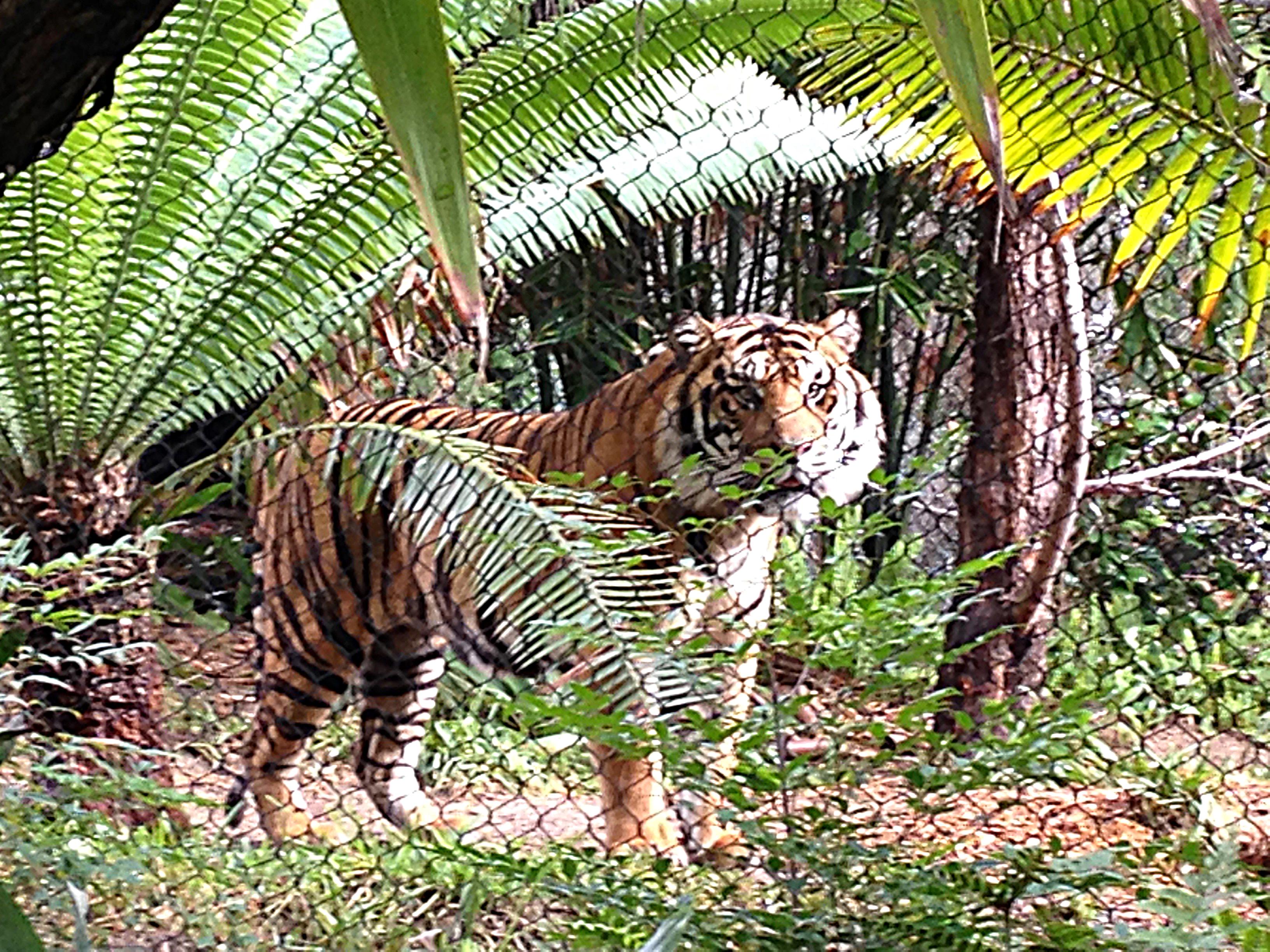
Here are a few of my favorites:
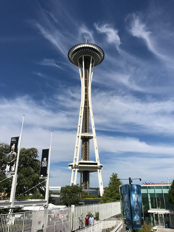
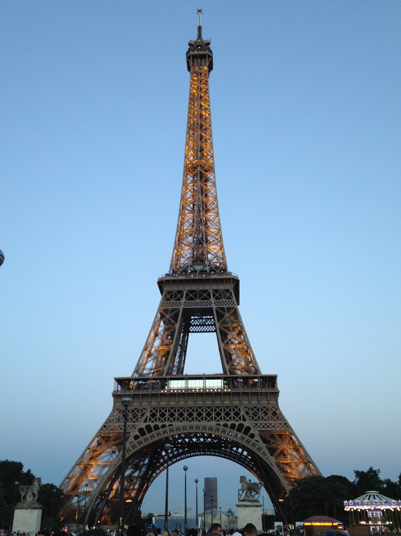
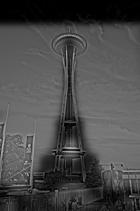
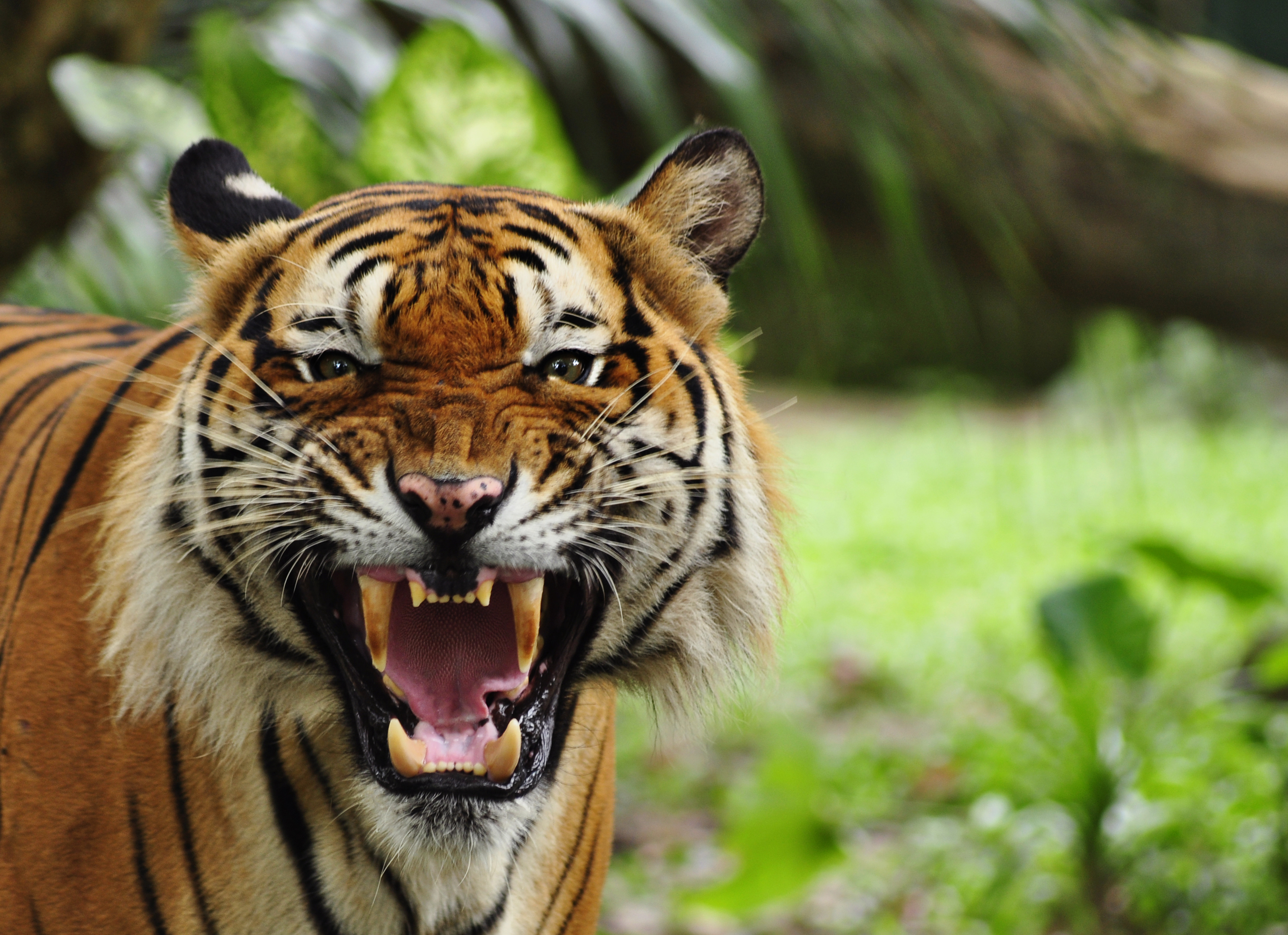
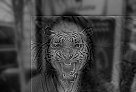
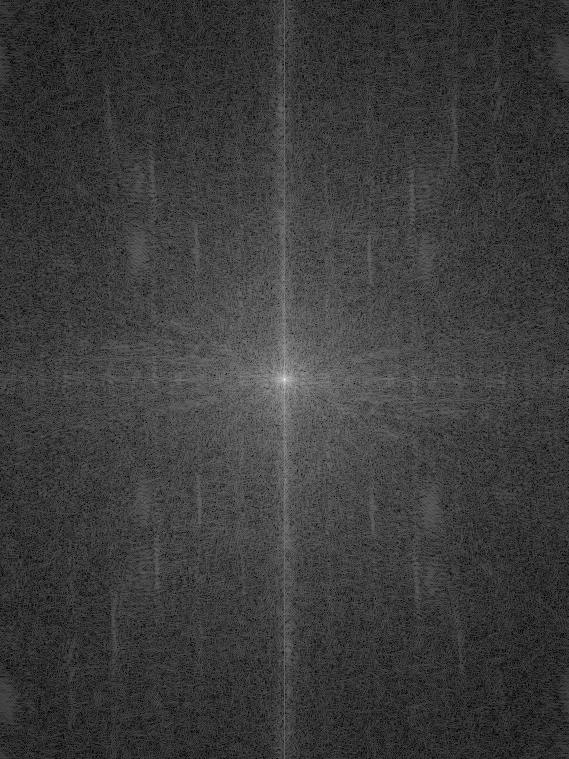
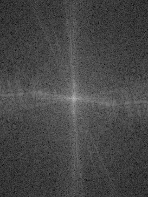
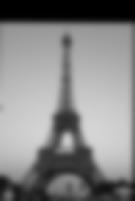
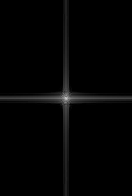
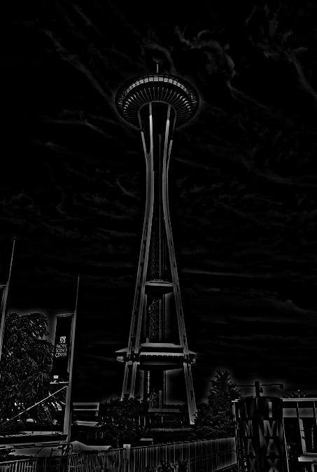
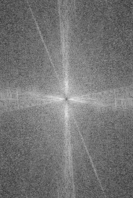
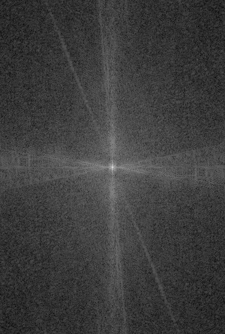
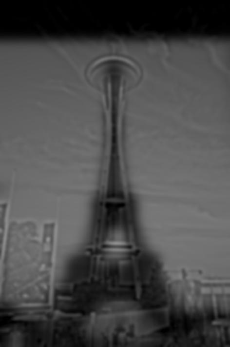
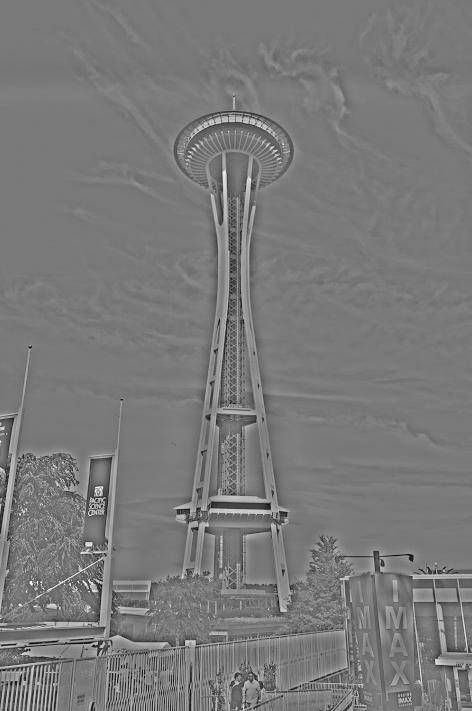
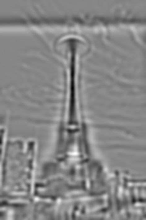
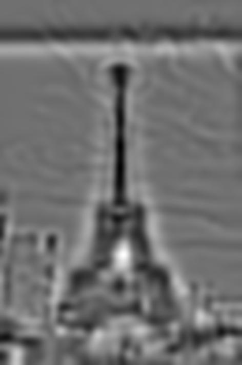
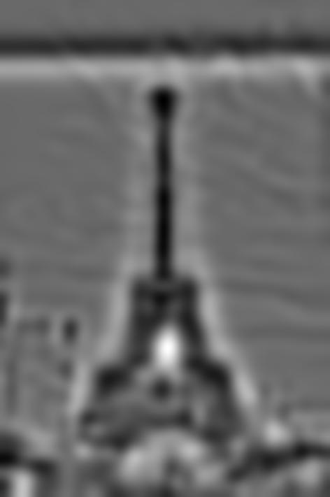
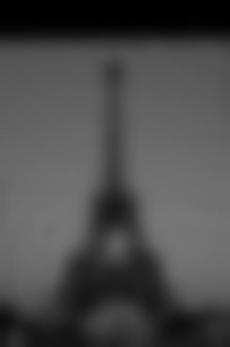
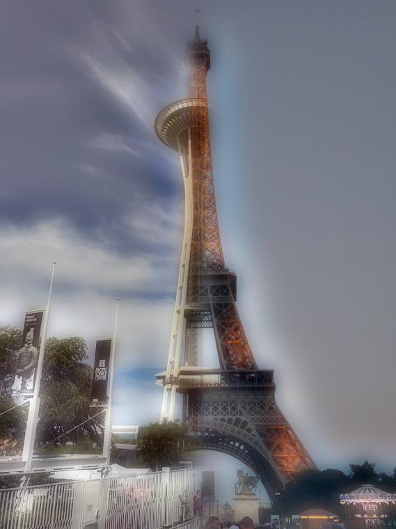
I decided to do a Fourier analysis for the images relating to the Space Needle/Eiffel Tower hybrid image. Below I have displayed an image followed by the log magnitude of the Fourier transform of that image.
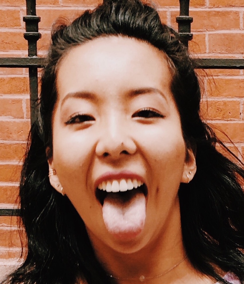
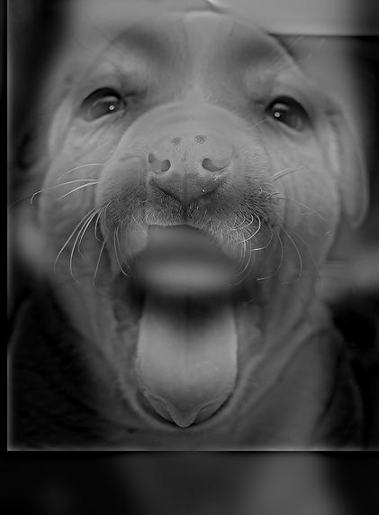
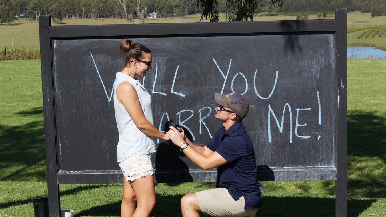
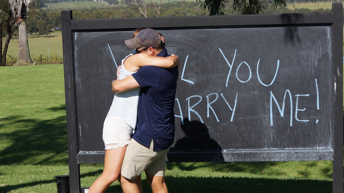
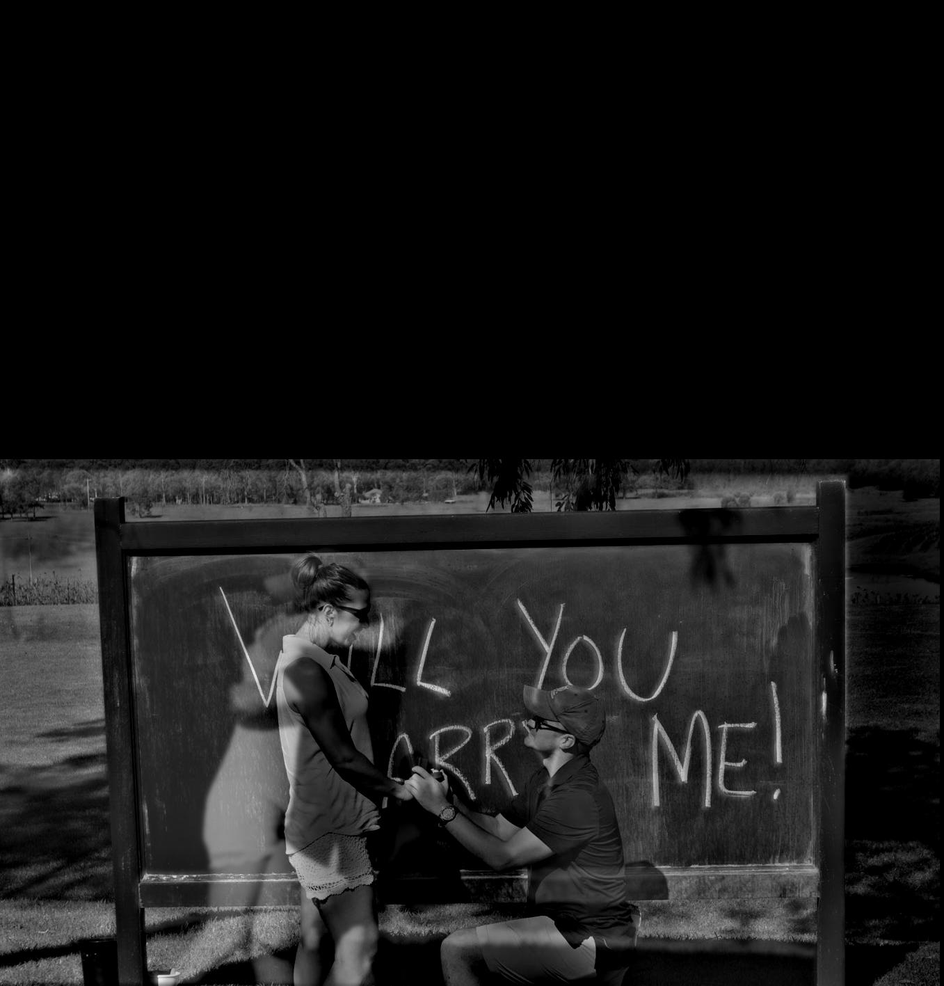
I tried to create a hybrid image of my cousin's proposal (before and after she said yes), but as you can see, the lack of alignment in their bodies makes it so that the result is not quite a hybrid image, but instead looks like an image with two ghosts at whatever distance it is viewed at.
For this part of the project, I implemented Gaussian and Laplacian stacks. To implement Gaussian
stacks, I took an image, then applied a Gaussian filter to that image to produce a result. I
then applied a Gaussian filter to that result, and continued that process for the specified number
of levels in the stack. To implement the Laplacian stack, each level of the Laplacian stack was the
difference between two levels in the Gaussian, with the exception of the last level of the Laplacian
stack, which was equal to the last level in the Gaussian stack. The motivation behind this is so that
superimposing all images in the Laplacian stack will result in the original image.
Here is an example of an image that I applied the Gaussian and Laplacian stacks to:
For this image, I used 5 levels for each stack, with a sigma value of 3.
Gaussian Stack:


Laplacian Stack:
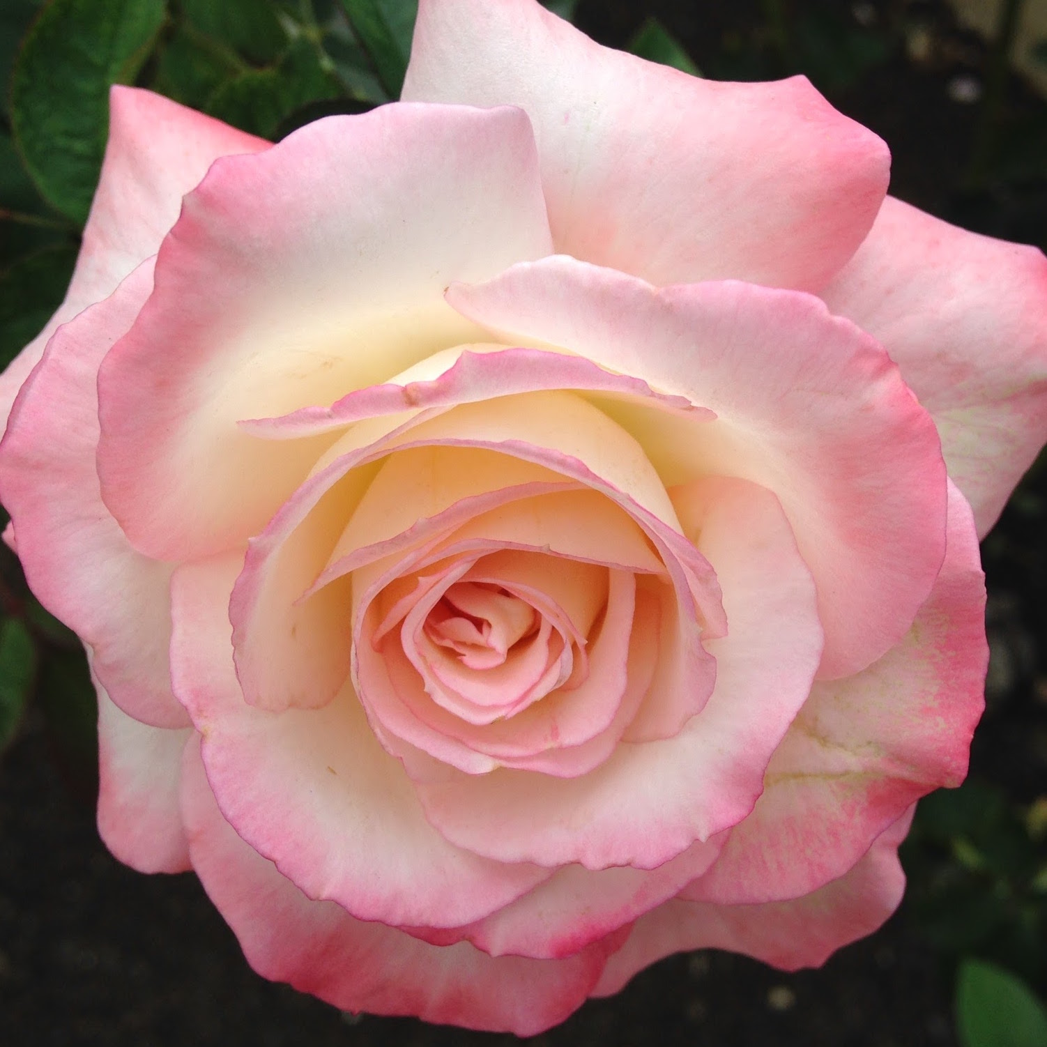
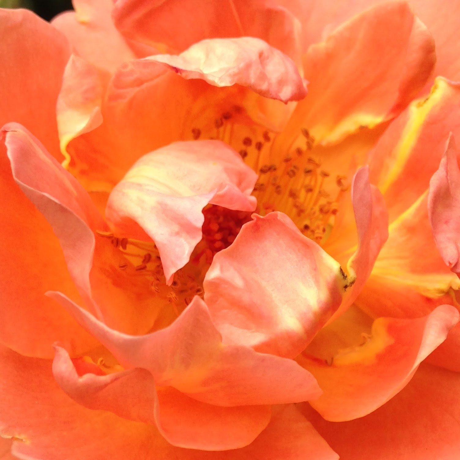
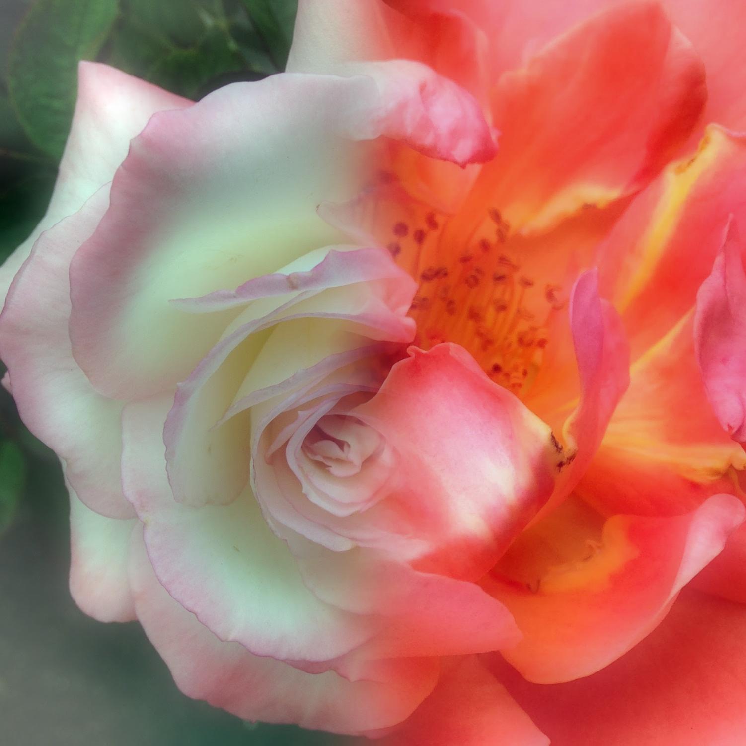
For this part of the project, we blended two images together. To determine which part of the image to blend, we created a mask for the image such that the pixels overlapping the areas of the image we wanted to include were set to 1, and the rest of the pixels were set to 0. Before processing the images, I split them into their separate RGB color channels, and did the processing to each channel. I calculated the Laplacian stack for both images, and the Gaussian stack for the mask. Then, for each layer of the stack, I multiplied the Gaussian of the mask with the Laplacian of one image and added it to the product of the compliment of the Gaussian of the mask and the other image. After completing this for each level of the stack, I added the results for all the layers together, normalized the final results, and combined the color channels together to make one smoothly-blended and colored image! I used 5 levels for the stacks, and used different values of sigma depending on the image choices. Here are some of my favorites:
For this part of the project, we had to compute the gradients of an image, and then use these calculated gradients and a pixel value as a boundary constraint to reconstruct this image. We did this by writing these gradients and the pixel value as a system of linear equations which we then solved by using the Least Squares approximation. The resulting image was the closest solution to that system of linear equations - which means it was essentially identical to the original image itself!
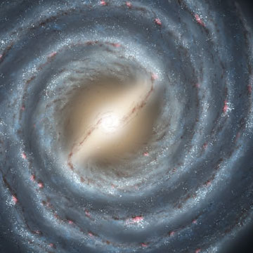
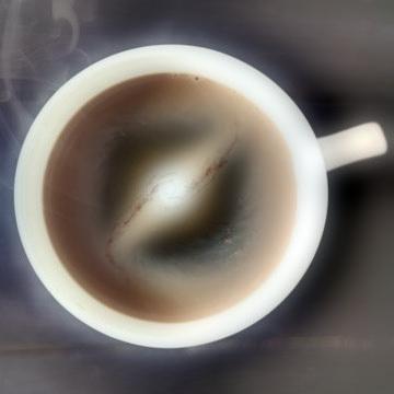
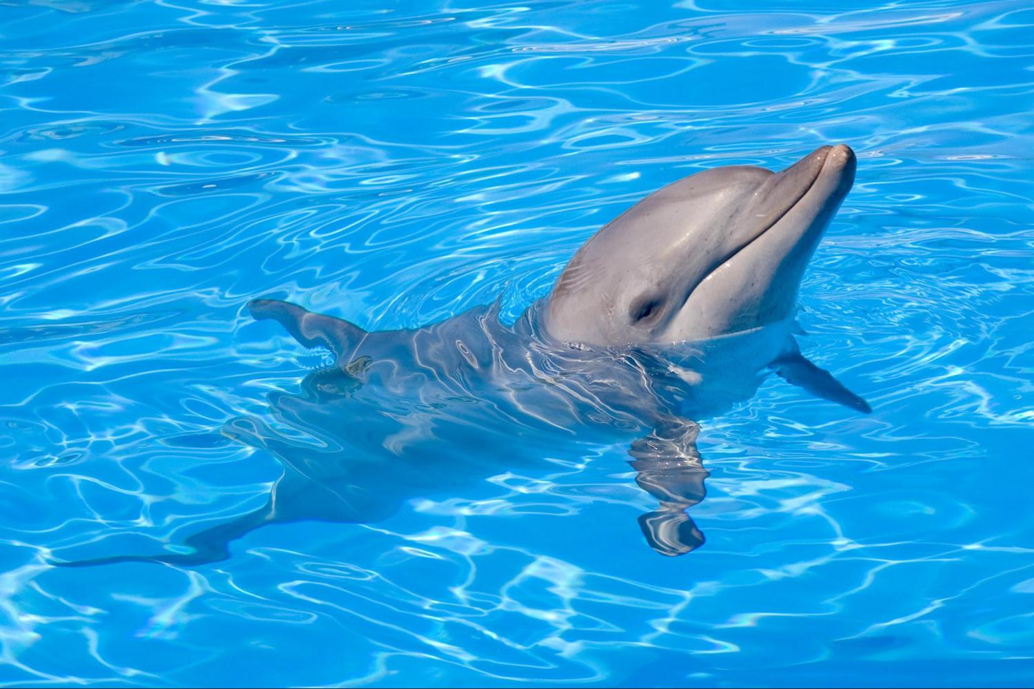
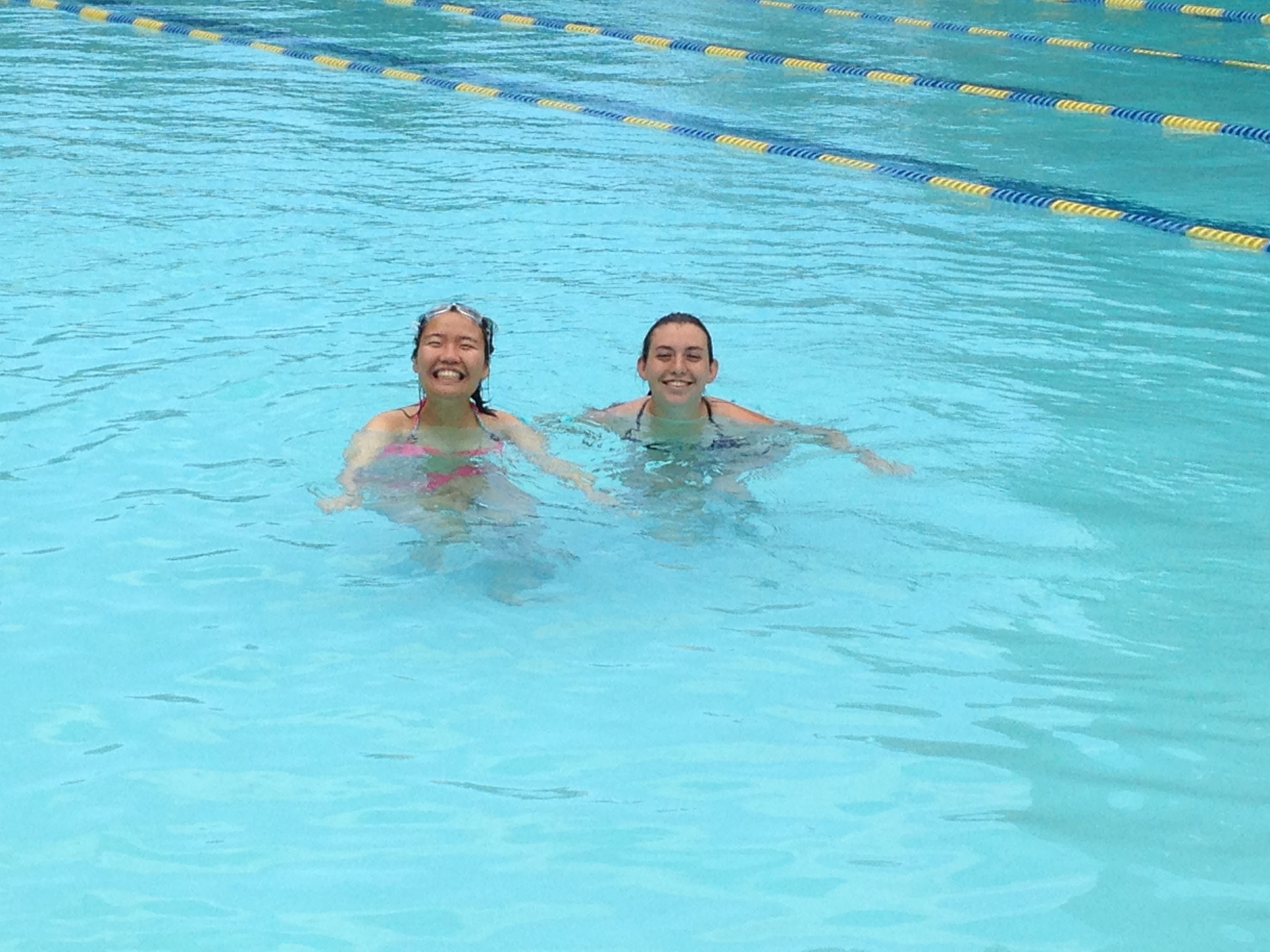
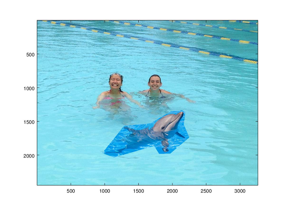
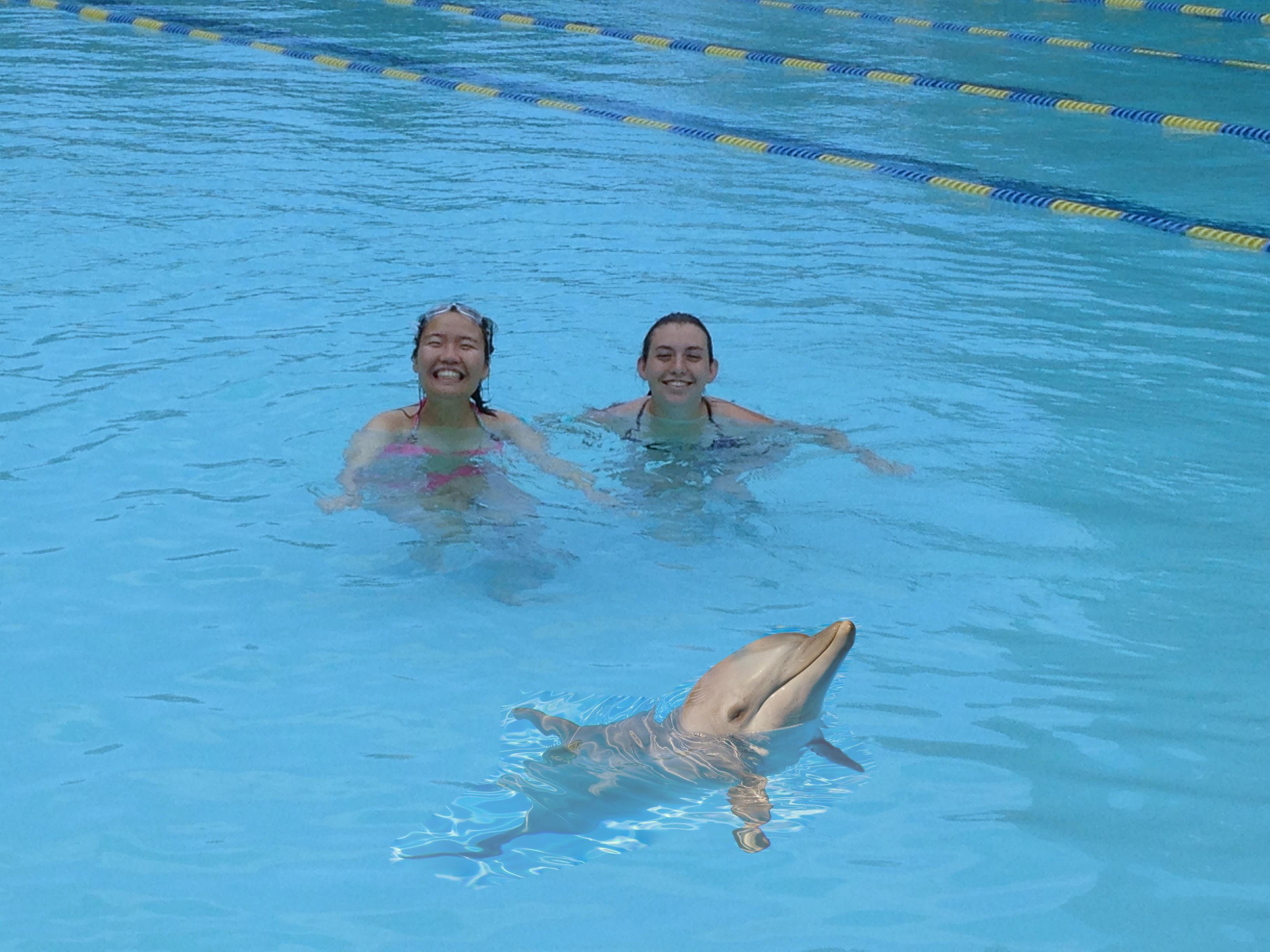
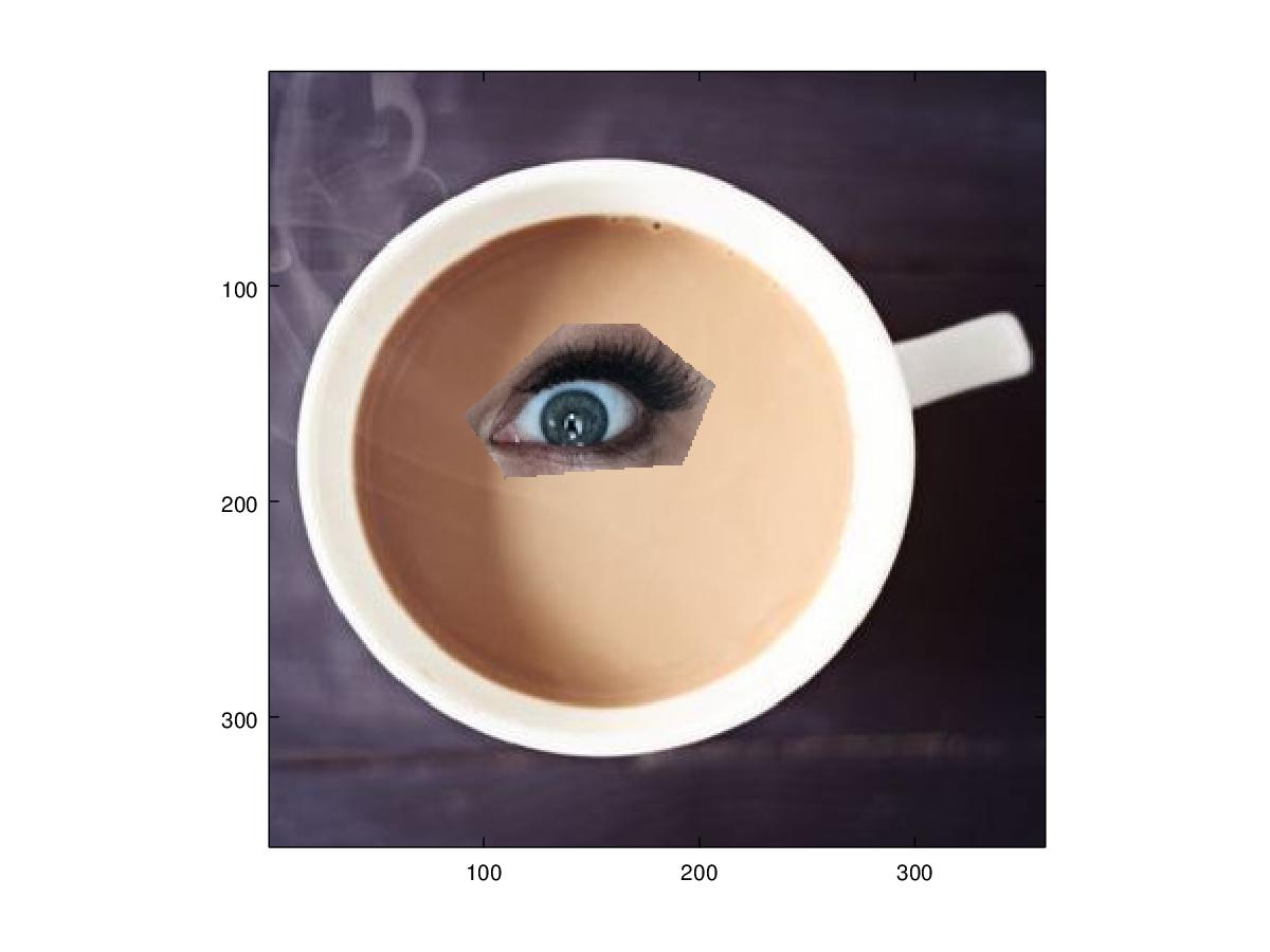
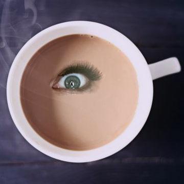
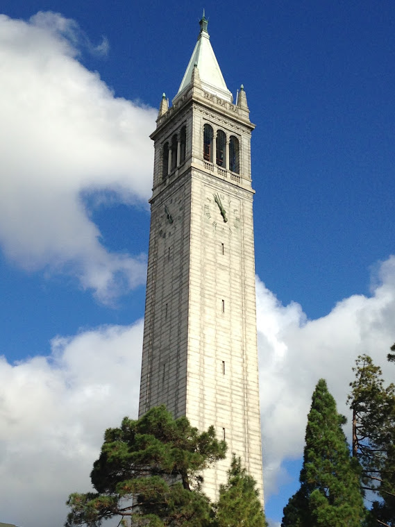
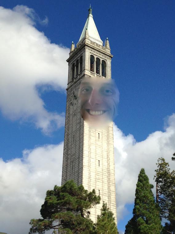
For this part of the project, we blended an image (the source image) onto another background image (the target image). The first step for combining these images was to create a mask that included only the piece of the source image we wanted to copy over, and to create a new source image that placed that piece of the image in the place that we wanted it to be in the target image. I used the provided Matlab code to take care of this step. Then, using this mask and generated source image, I set up a system of linear equations (like in the previous problem). My goal was to have the gradients of the source image within the mask be equal to the gradients in the final image, and for the boundary pixel values of the mask to match the pixel values of the target image. I translated these constraints into a system of linear equations, and then determined the resulting image by finding the Least-Squares approximation to the system of equations (as this is the best approximation to the constraints we desire). In the resulting image, you should not be able to tell which part of the image came from the source, and which came from the target! Here are a few of my favorite examples:
Failure Explanation
As you can see, this combination did not work very well. One reason for this is that preserving the
gradients of the source image results in any texture from the target image not being propagated.
This creates a more obvious border, as you can clearly see where the texture of the bricks ends.
Another reason that this combination did not work well is that the face crosses over an edge - in this
case, it was the edge between the Campanile and the sky. There are boundary conditions for both
of these, which creates conflicting constraints that the face tried to satisfy. This resulted in the
face propagating some of the blue sky color into the Campanile, and overall adopting a color that did
not quite blend.
Laplacian blending is better in the situation where you want to more closely preserve the source image
colors, or when the source image is being placed in an area that crosses over an edge separating distinct
colors. Laplacian blending blurs the borders between images, so it would not be good for cases in which you
want to preserve the image detail around the border. This is also good for images in which there is a texture
shift across boundaries, because the blurring will make this transition smoother.
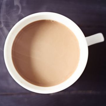
Poisson blending is better in the opposite scenarios. The use of boundary constraints causes the
source image to adopt the colors of the target image, so Poisson blending would be prefered if you do not
need the colors of the source image to be preserved. Because Poisson blending aims to preserve the gradients
of the source image, Poisson blending is good for images in which you would like to preserve the detail of
the source image and do not mind the colors being shifted. However, Poisson blending is not very successful in
combinations of images where the texture is very different across the border, because preserving the gradients
preserves the difference in texture, and it will make a very obvious boundary.

As you can see, Poisson blending resulted in the galaxy adopting more of the colors of the coffee, whereas the Laplacian blending resulted in the galaxy maintaining more of its own color. I think that both approaches worked for this combination of images, but I personally prefer the Laplacian blended image in this case.