Part 1.1 - Warmup
Overview
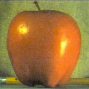
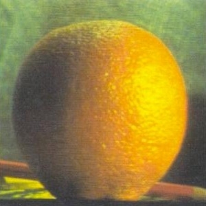
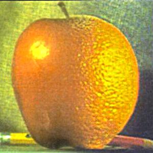
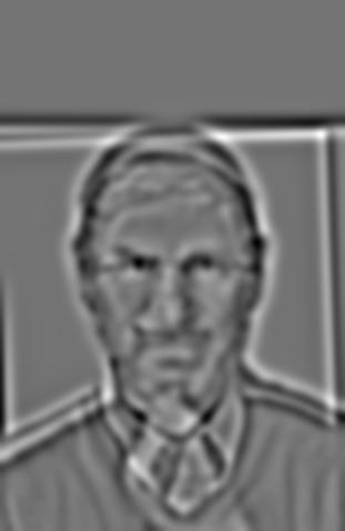
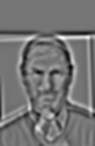
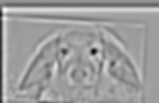
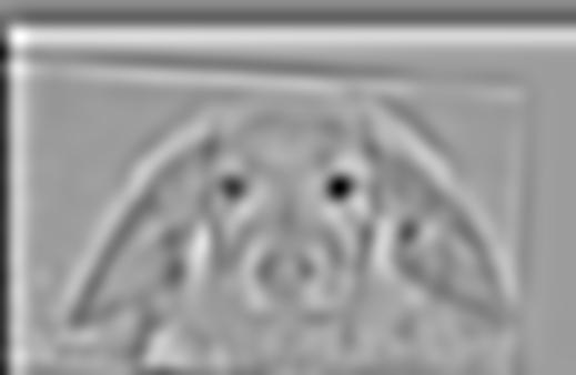
For image sharpening, I used the unsharpen masking technique from class, where
Sharpened image = f + α(f − f * g) = f * ((1+α)e −αg)
In my case, α = 1.5, and f * g was simply the original image convoluted with a gaussian filter with sigma = 5. Sharpening was performed only on grayscale images.
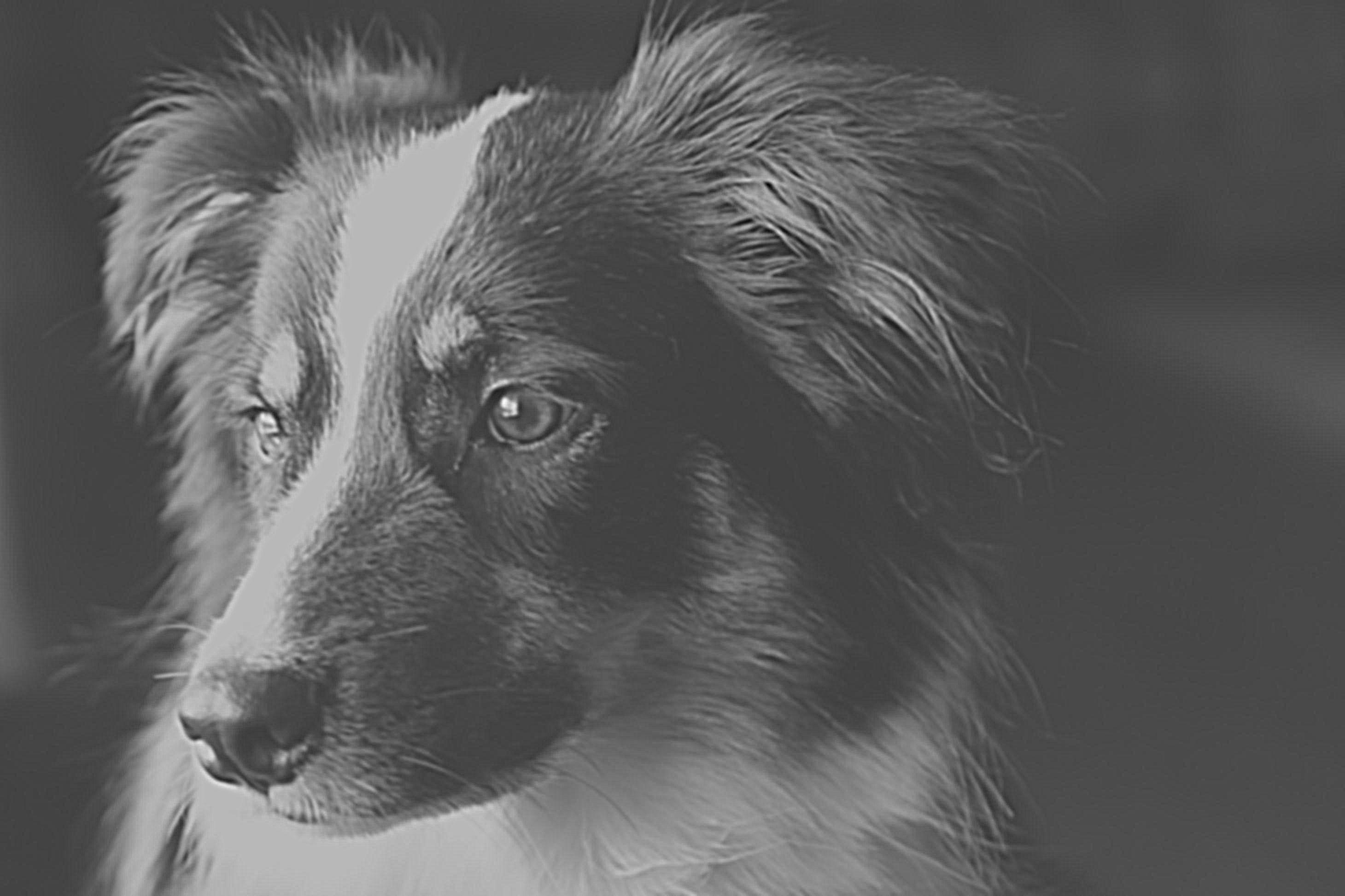
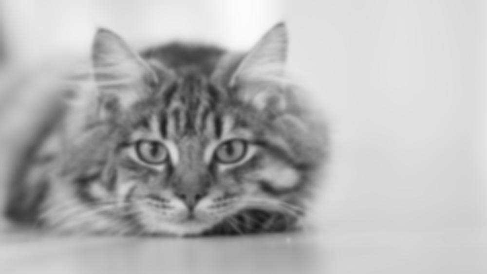 Before Sharpen
|
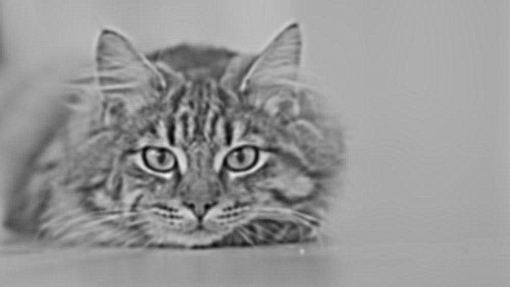 After Sharpen
|
 Before Sharpen
|
 After Sharpen
|
Part 1.2 - Hybrid Images
Overview
To generate hybrid images, I followed the approach described in the SIGGRAPH 2006 paper: to combine the low frequencies of one image with the high frequcies of another image. Using gaussian filters, I first applied a low pass filter with sigma = 3 to the first image, then I applied a high pass filter with sigma = 10 to the second image. The resulting low frequency and high frequency images are then combined. Note that image alignment is done by aligning the eyes.
Hybrid image of Derek and Nutmeg
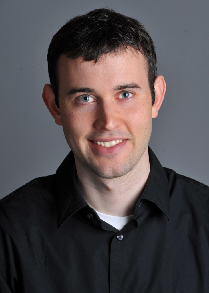 Derek
Derek
|
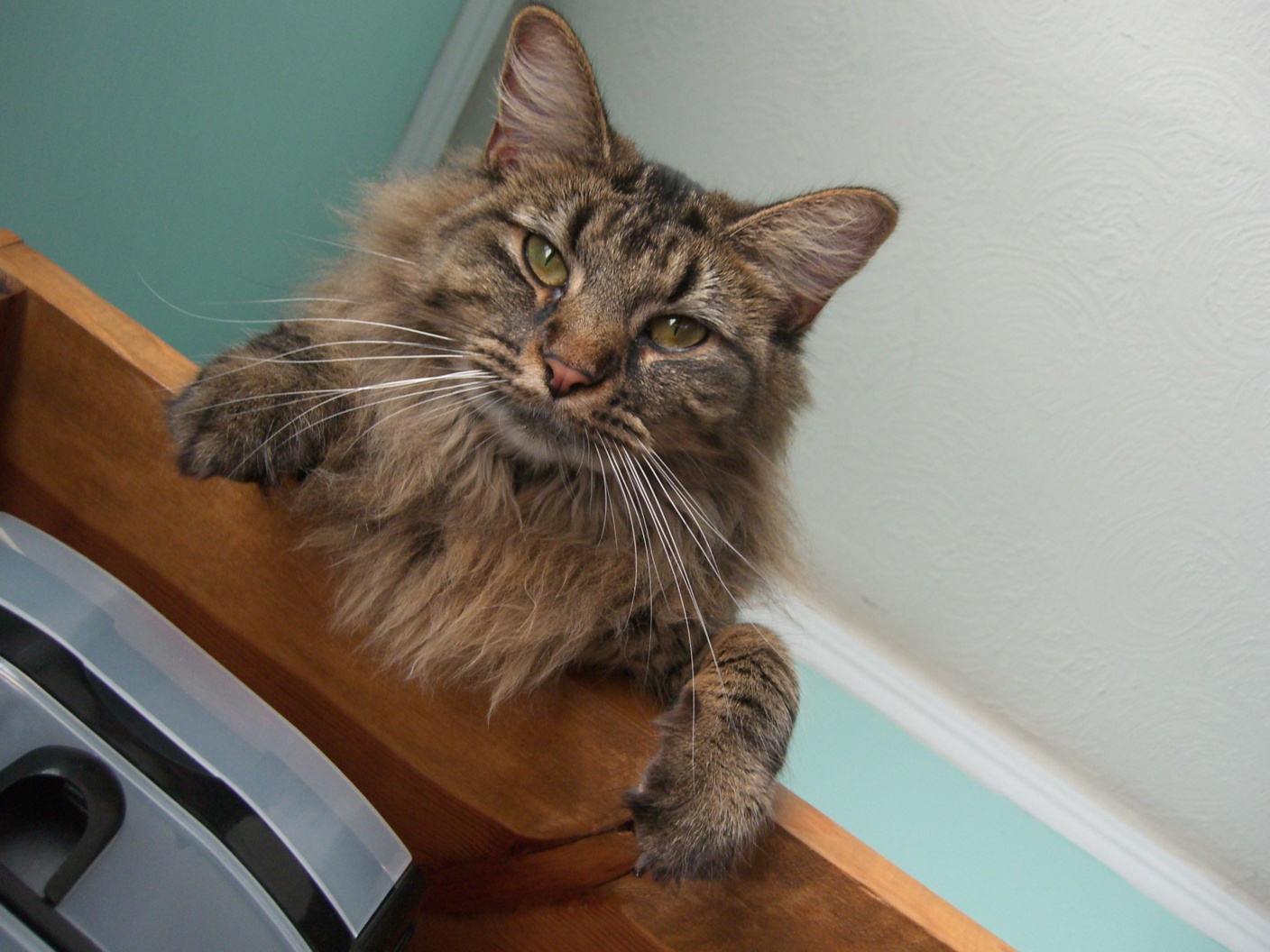 Nutmeg
|
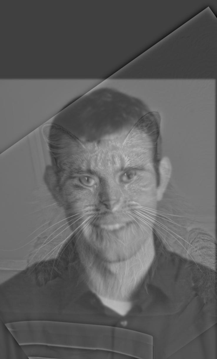 Hybrid Image
|
Hybrid image of Steve Jobs and Bill Gates (Favorite)
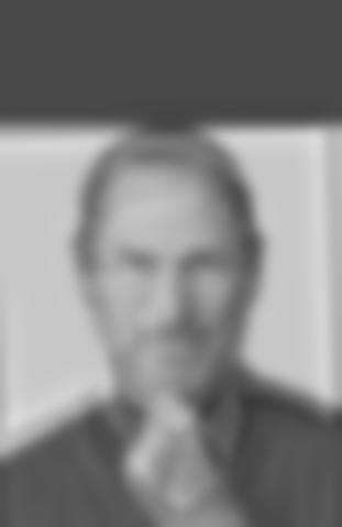
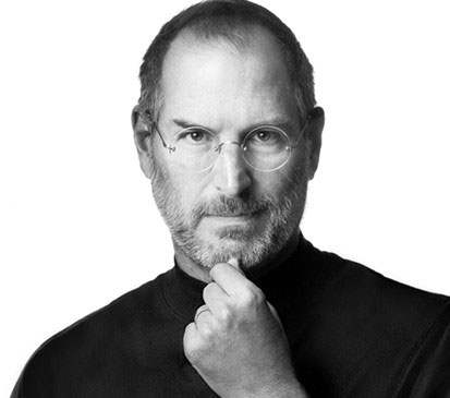 Steve Jobs
|
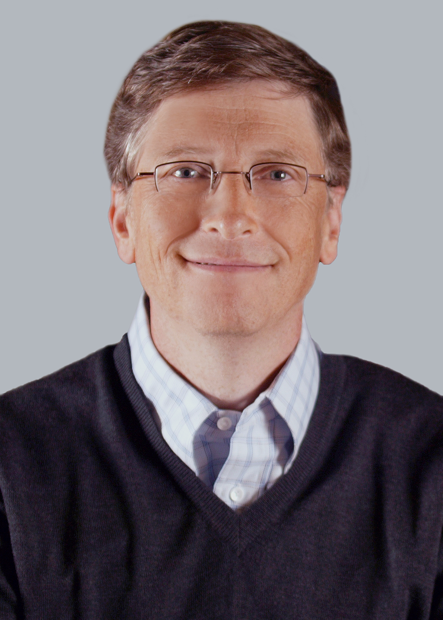 Bill Gates
|
 Hybrid Image
|
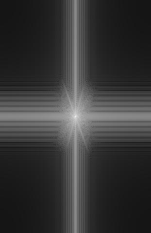
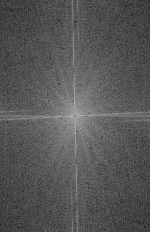
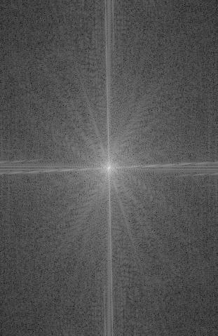
Frequency analysis of Steve Jobs and Bill Gates images
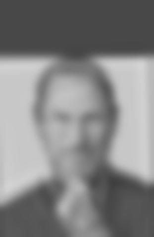
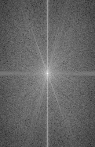 Steve Jobs original image
|
 Steve Jobs low frequency
|
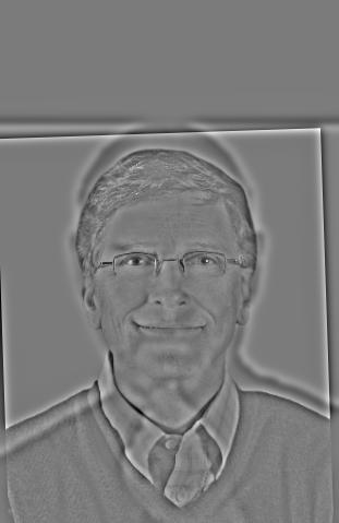
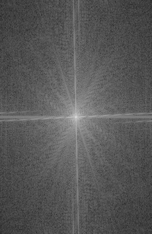 Bill gates original image
|
 Bill gates high frequency
|
 Hybrid
|
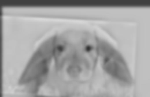
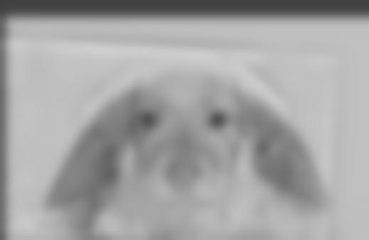
Hybrid image of a bunny and a puppy
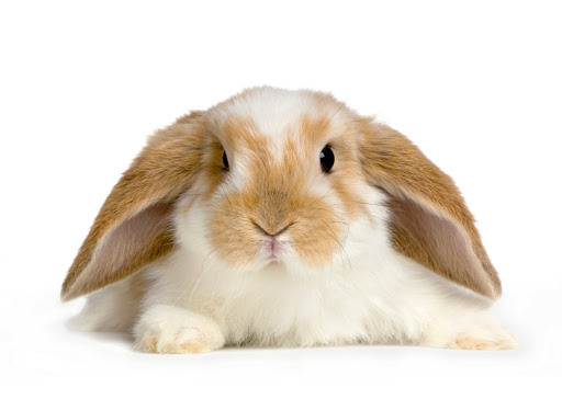 Bunny
Bunny
|
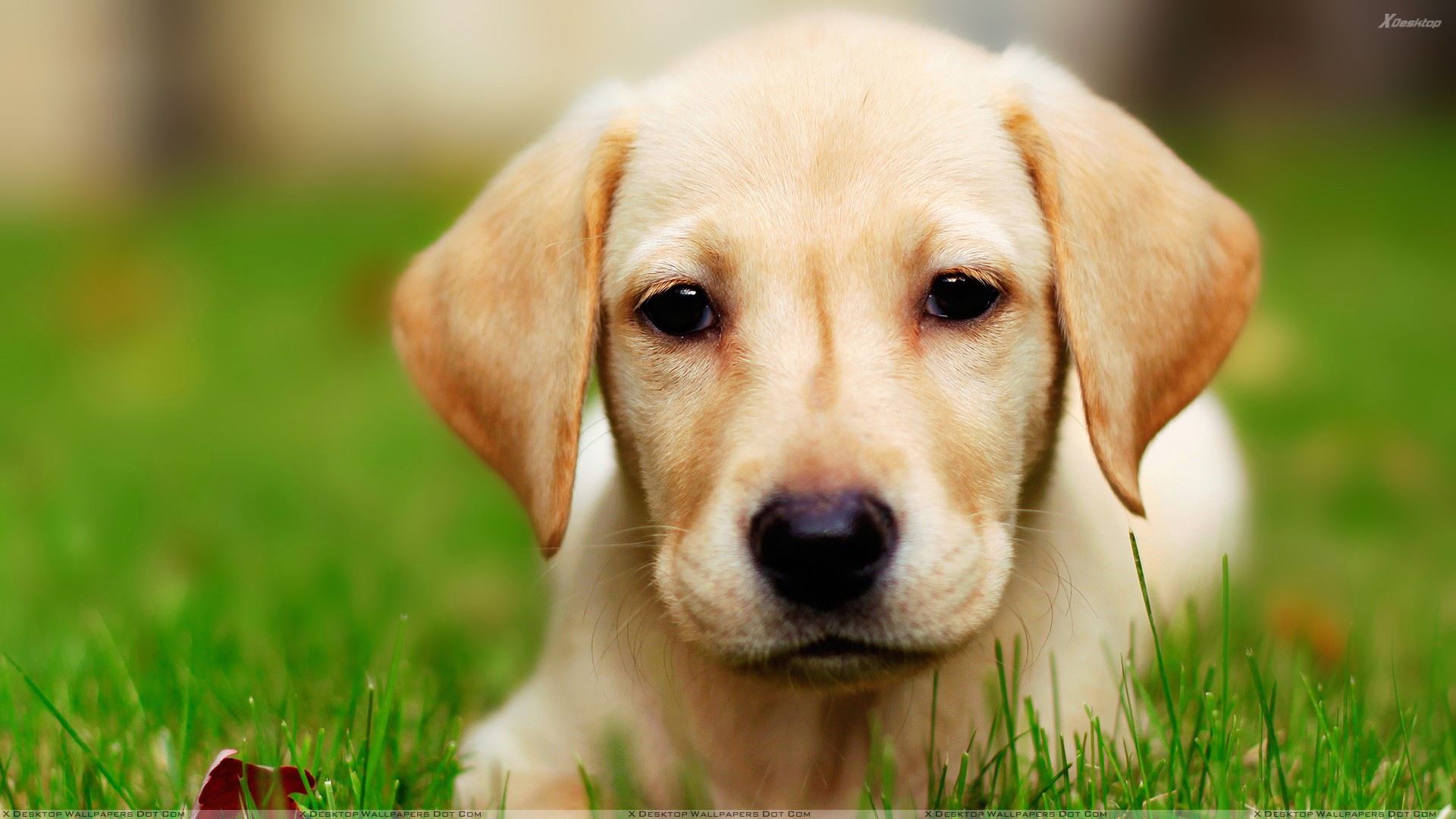 Puppy
Puppy
|
 Hybrid Image
|
This one didn't work too well...
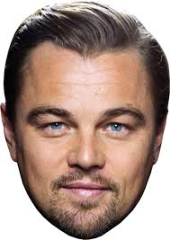 Leonardo DiCaprio
|
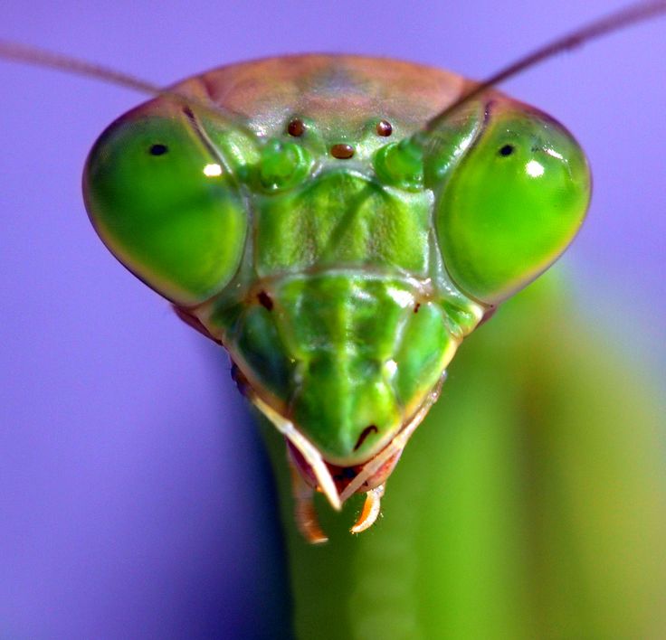 Mantis
|
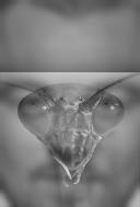 Hybrid Image
|
Most of the hybrid images turned out quite well, except for the hybrid image of Leonardo DiCaprio and the mantis. This is mostly because of the shape difference between a human face and a mantis' head. Even though their eyes match up, there is really no way to match the nose, mouth, cheeks, and other parts of the face.
Part 1.3 - Gaussian and Laplacian Stacks
Overview
Gaussian stacks are generated by repeatedly applying the gaussian filter at each level of the stack without downsampling the image to generate the next gaussian stack layer. Generating a laplacian stack involves taking the difference between the current and previous gaussian stack layers. For this part, I used a gaussian filter with sigma = 4 to generate the stacks.
Gaussian stack for the Lincoln and Gala painting
 Layer 0
|
 Layer 1
|
 Layer 2
|
 Layer 3
|
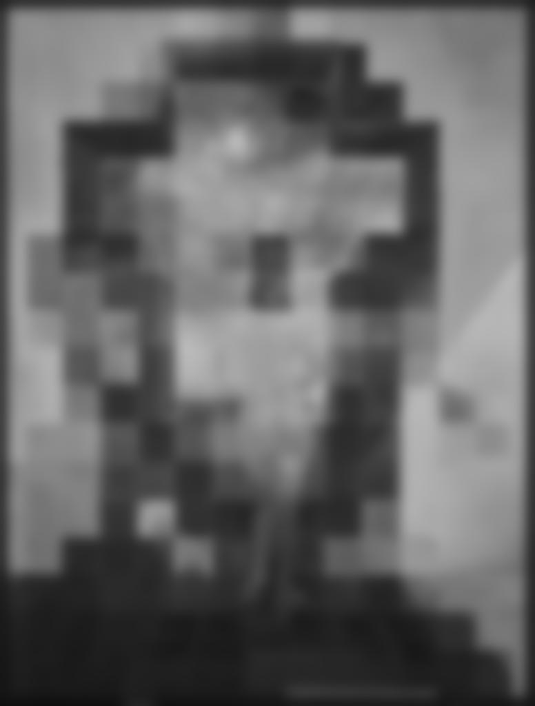 Layer 4
|
Laplacian stack for the Lincoln and Gala painting
 Layer 0
|
 Layer 1
|
 Layer 2
|
 Layer 3
|
 Layer 4
|
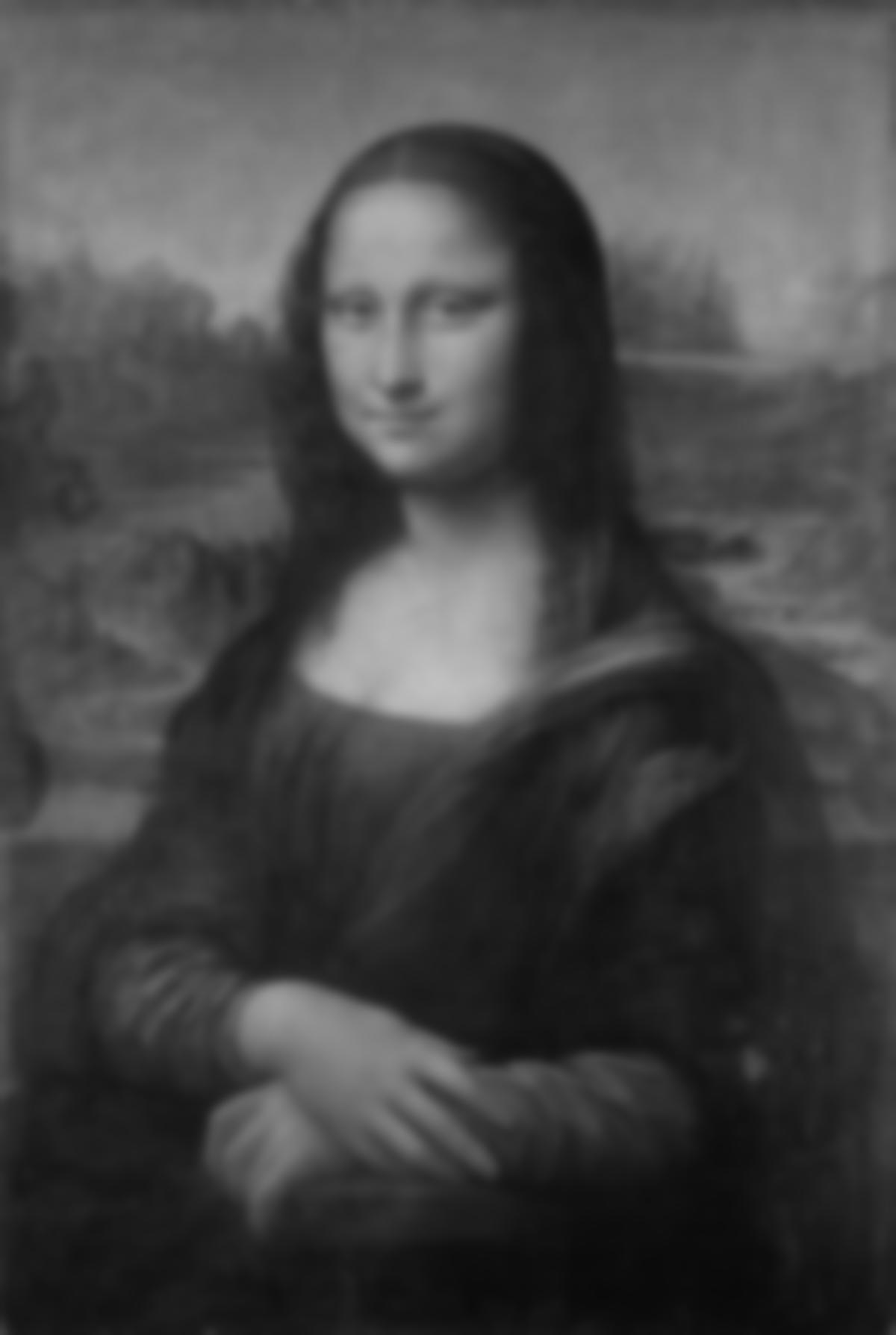
Gaussian stack for Mona Lisa
 Layer 0
|
 Layer 1
|
 Layer 2
|
 Layer 3
|
 Layer 4
|
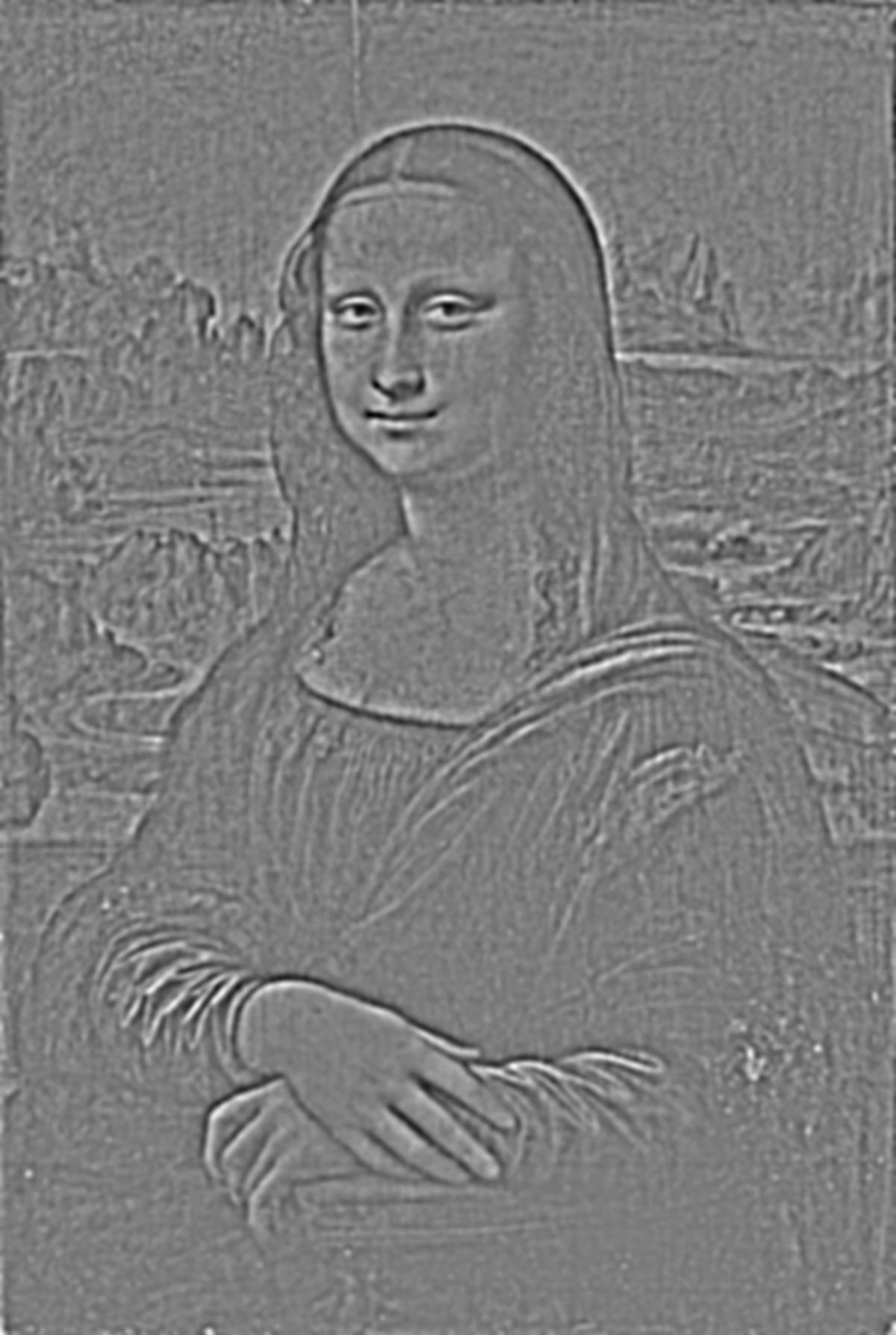
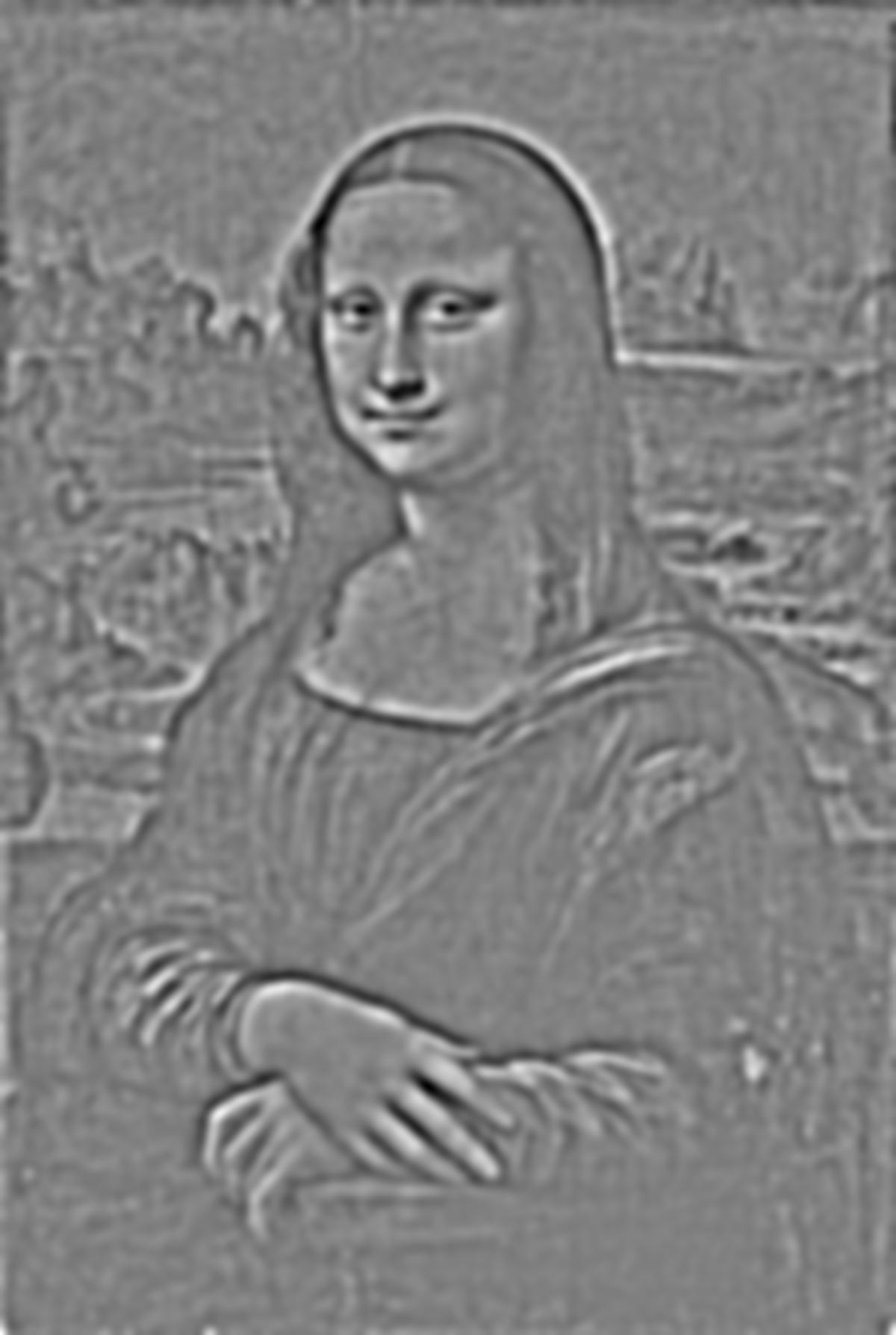
Laplacian stack for Mona Lisa
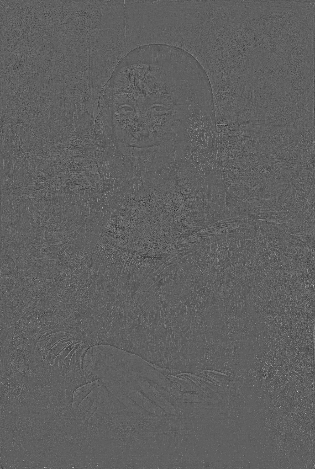 Layer 0
|
 Layer 1
|
 Layer 2
|
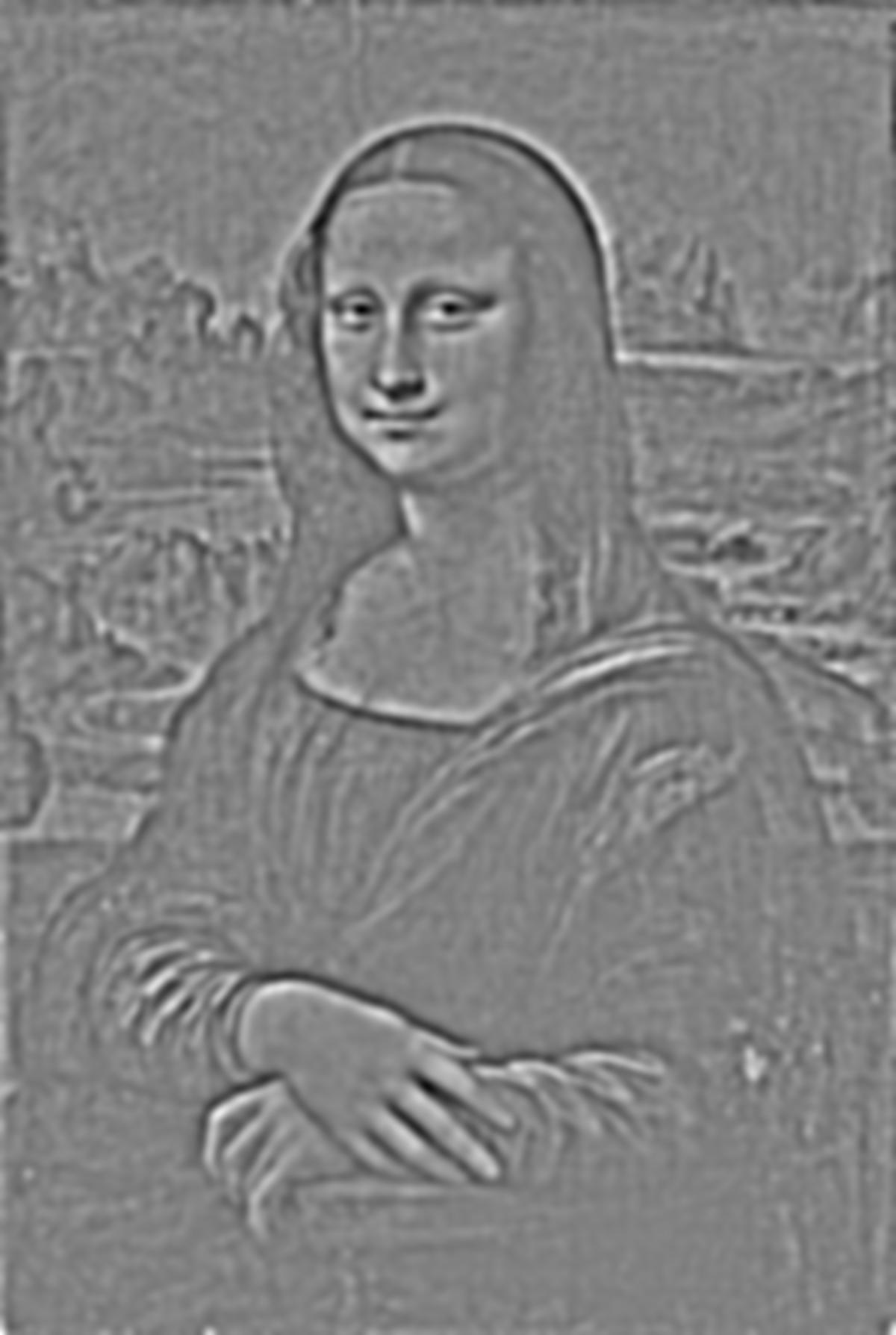 Layer 3
|
 Layer 4
|
Gaussian stack for Bill Gates and Steve Jobs Hybrid Image (Favorite)
 Layer 0
|
 Layer 1
|
 Layer 2
|
 Layer 3
|
 Layer 4
|
Laplacian stack for Bill Gates and Steve Jobs Hybrid Image (Favorite)
 Layer 0
|
 Layer 1
|
 Layer 2
|
 Layer 3
|
 Layer 4
|
Here's another stack...
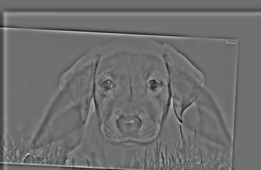
Gaussian stack for Bunny and Puppy Hybrid Image
 Layer 0
|
 Layer 1
|
 Layer 2
|
 Layer 3
|
 Layer 4
|
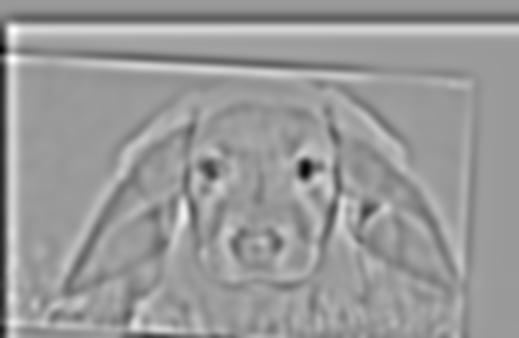
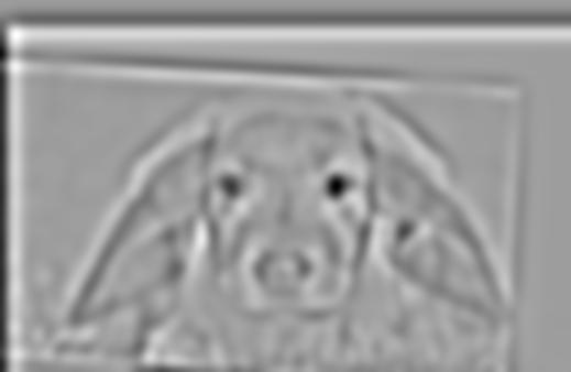
Laplacian stack for Bunny and Puppy Hybrid Image
 Layer 0
|
 Layer 1
|
 Layer 2
|
 Layer 3
|
 Layer 4
|
Part 1.4 - Multiresolution Blending
Overview
For this part, two images are blended seamlessly together using the multiresolution blending technique in Burt and Adelson's 1983 paper. The idea is to create a laplacian and gaussian stack for both input images, as well as a gaussian stack of the mask. The gaussian stack of the mask is used to smooth out the edges between the 2 images and is combined with the laplacian and gaussian stacks of the input images at each stack level to result in a stack of blended images. The layers of this stack are summed together to create a seamlessly blended output image. Note that my laplacian stack used a gaussian filter with sigma = 1, my gaussian stack used a gaussian filter with sigma = 2, my mask stack used a gaussian filter with sigma = 20, and my irregular mask stack used a gaussian filter with sigma = 5. I found that these sigma values produced the best results.
Part 2 - Gradient Domain Fusion
Description
Part 2 of the project focuses on Poisson Blending to seamlessly blend an object or texture from a source image to a target image. Since people often care more about the gradient of an object than the overall intensity, the goal of Poisson Blending is to find values for image pixels that can preserve the source image's gradients as much as possible without changing any background (target) pixels. After all, even if the intensity of 2 blended images matches, if the colors don't match up, then the seam is easily noticable. Using least squares, we want to minimize the gradient differences in the area being blended between the source region and the new region we are creating, v, all the while minimizing the gradient differences between the source region, and the target and v regions at the boundaries of the region by formulating the problem as:

This objective function guides the new gradient values to match the gradient values of the source region, all the while allowing the gradient values of the background (target) region to propegate through the area of the source region via the edges of that region, allowing for smooth color transitions between image seams.
Part 2.1 - Toy Problem
Overview
For the toy problem, the x and y gradients of the original image is computed and a least squares problem is set up to minimize the x and y gradient difference between the gradient reconstructed image, v, and the original toy image. An additional constraint on the top left pixel intensity of both images is added as another objective to the least squares problem to preserve the overall intensity of the reconstructed image in respect to the original image. Solving this least squares problem and reshaping the vector gives us the pixel values of the reconstructed image v, which should be almost equivalent to the original toy image due to gradient and intensity preservation. In my case the calculated error is: ~0.0368
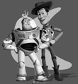 Original Image
|
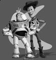 Reconstructed Image
|
Part 2.2 - Poisson Blending
Overview
For this part I first created irregular masks using saveMask.m (code provided by Jun-Yan on Piazza) and, as described in the part 2 description section, basically applied the least squares equation provided in the project spec. To reduce computation time, I limited the region we are solving for using matrix A and vector b to be a rectangular region that tightly encompasses the white area of the mask.
Favorite Result
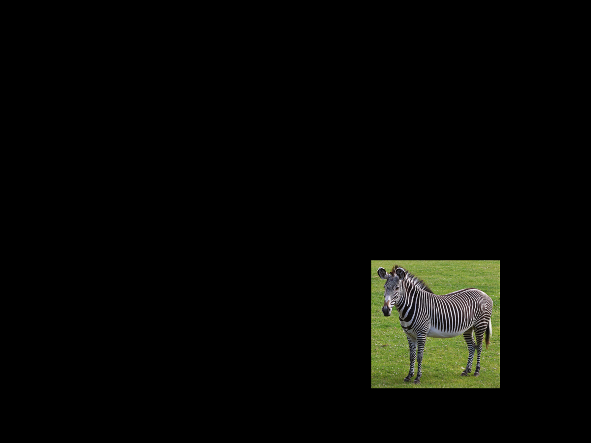 Zebra Source Image
|
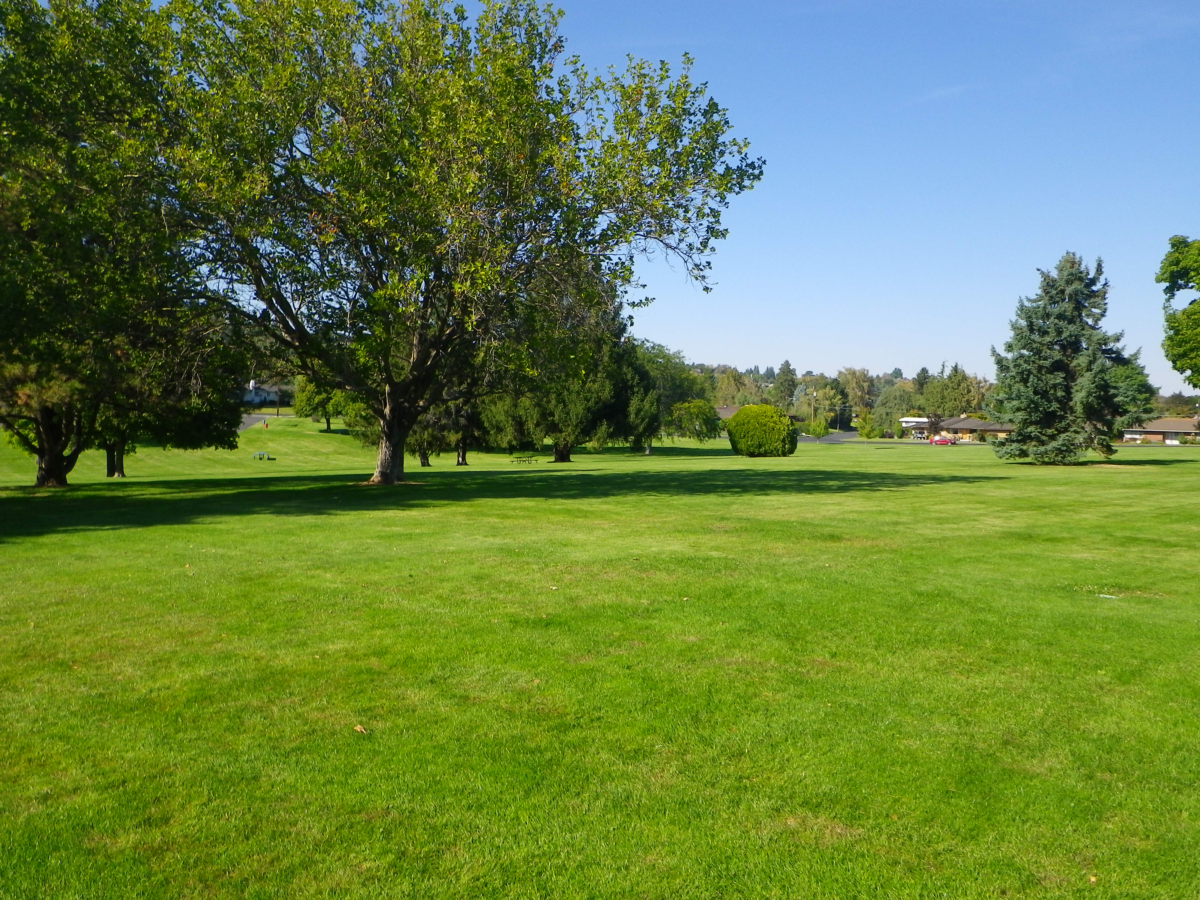 Park Target Image
|
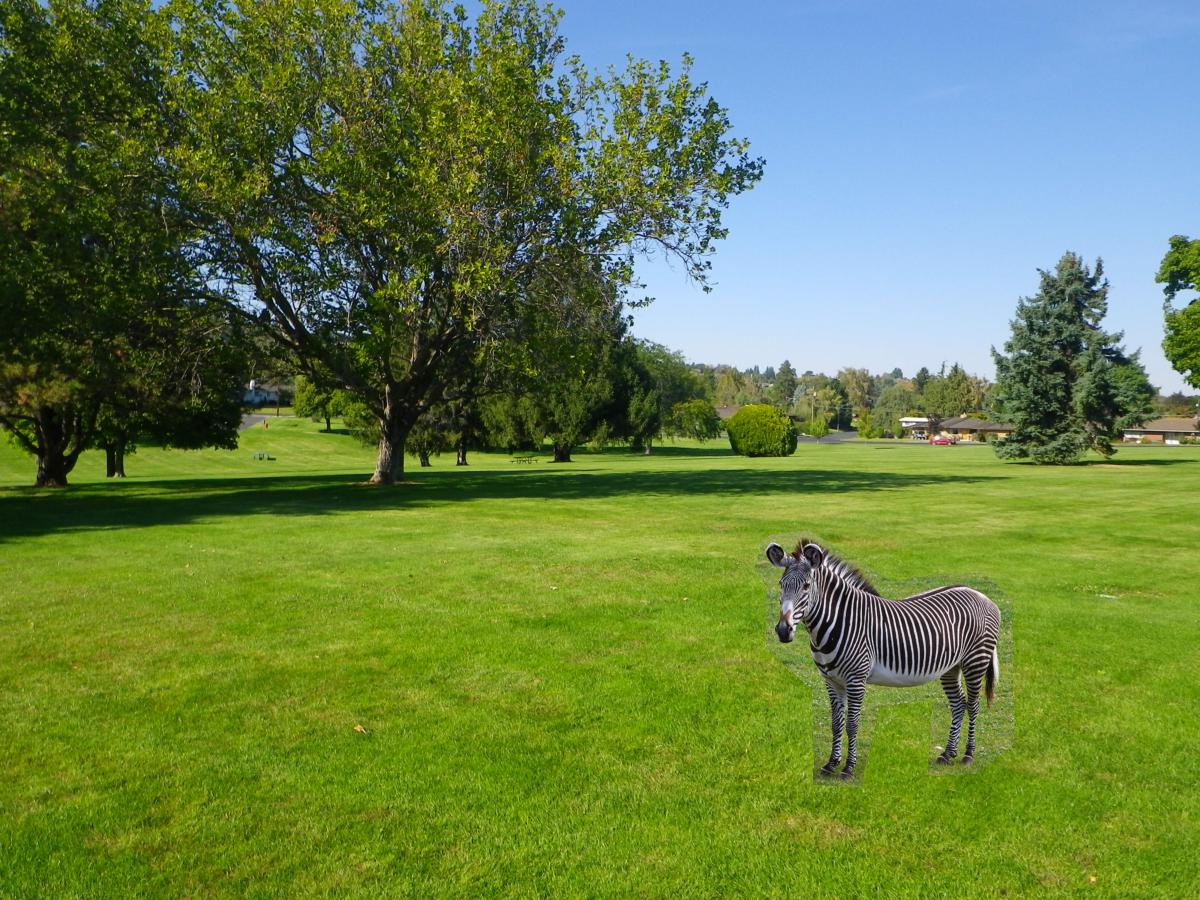 Source Pixels Directly Copied...
|
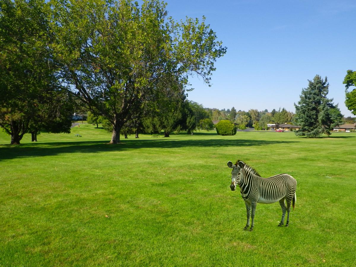 Final Result
|
Note that if we directly copy in source pixels to the target image, there is a distinct and noticable color difference at the seams. Also note that in the final image, the zebra's body turns slightly green, but its overall color balance between the white and black stripes does not deviate much from the original source image. This is because the gradients at each pixel of the source image is being preserved through the first part of the above least squares equation. The zebra turns green due to the second part of the least squares equation, which attempts to minimize the gradient difference at the boundary of the blended region, which causes the green color of the grass in the target image to creep in at the edges and propagate through zebra source image.
More Results...
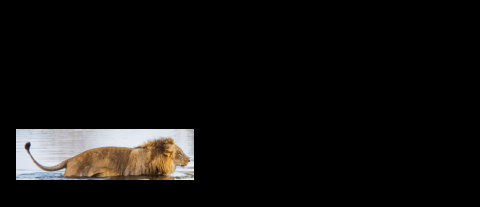 Lion Source Image
|
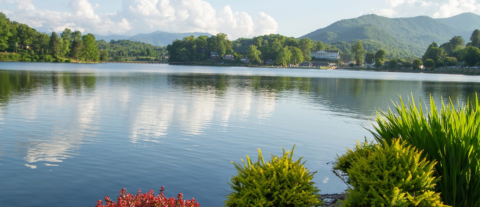 Lake Target Image
|
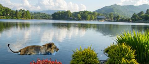 Final Result
|
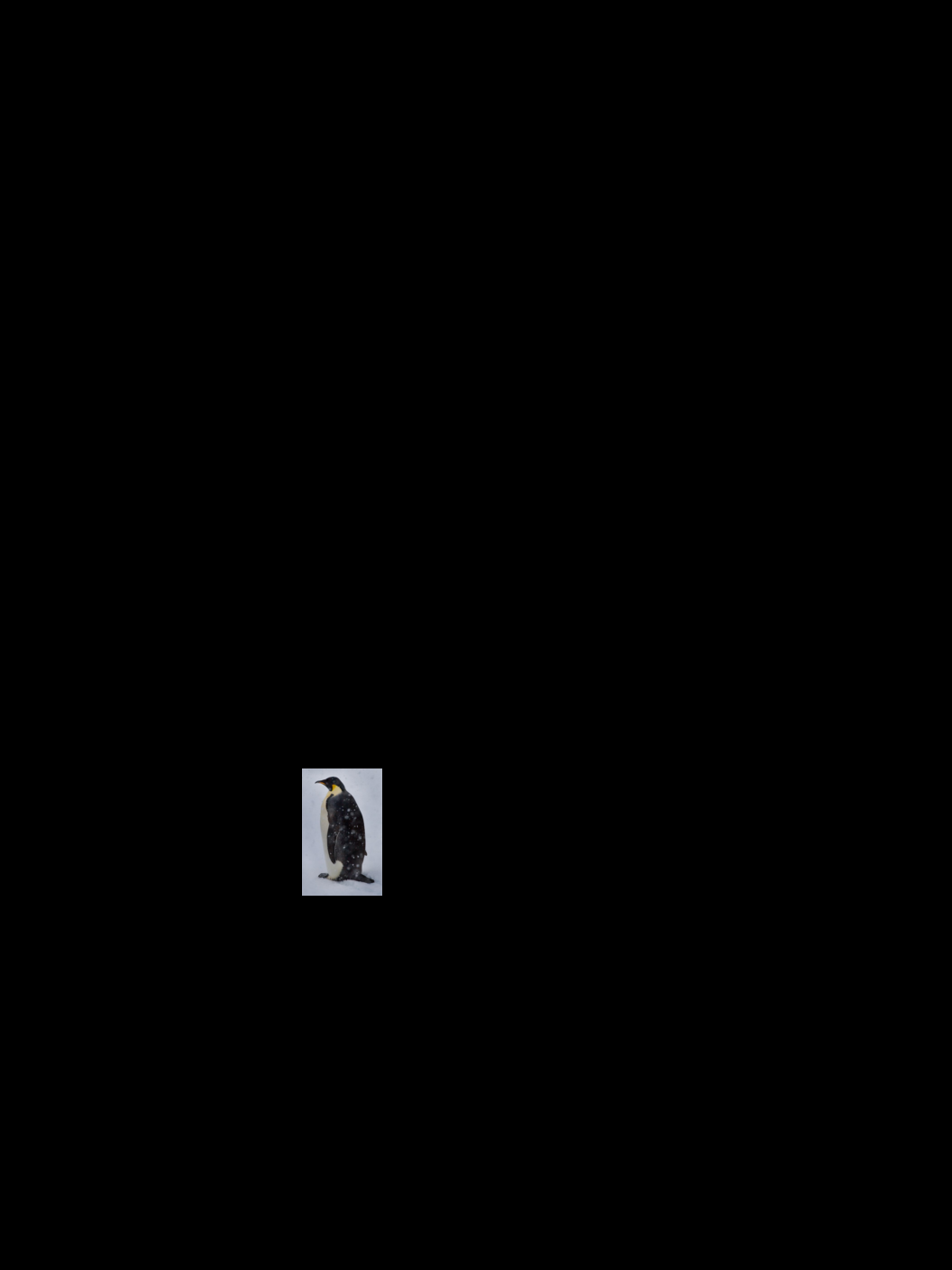 Penguin Source Image
|
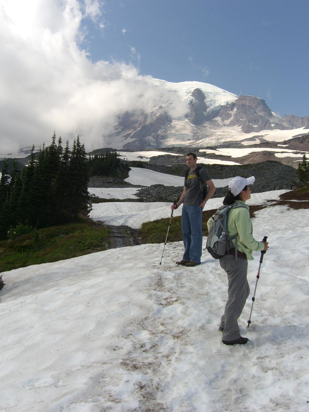 Snow Target Image
|
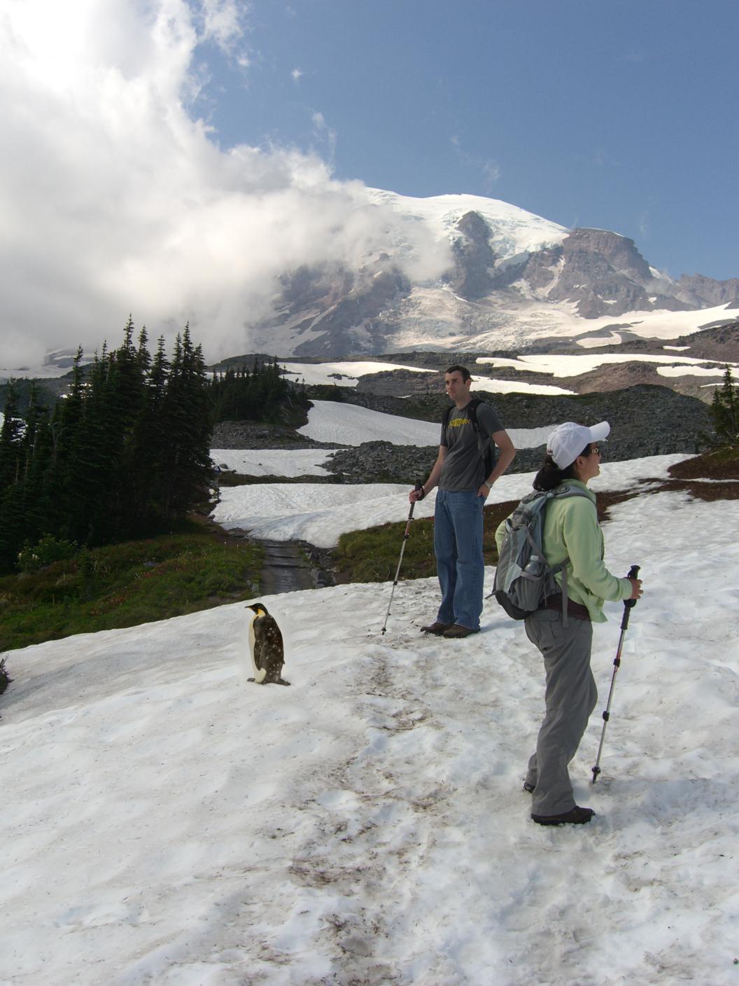 Final Result
|
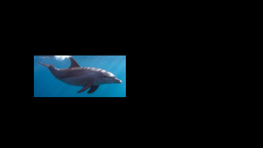 Dolphin Source Image
|
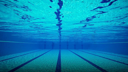 Pool Target Image
|
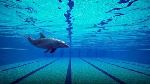 Final Result
|
Did not work so well...
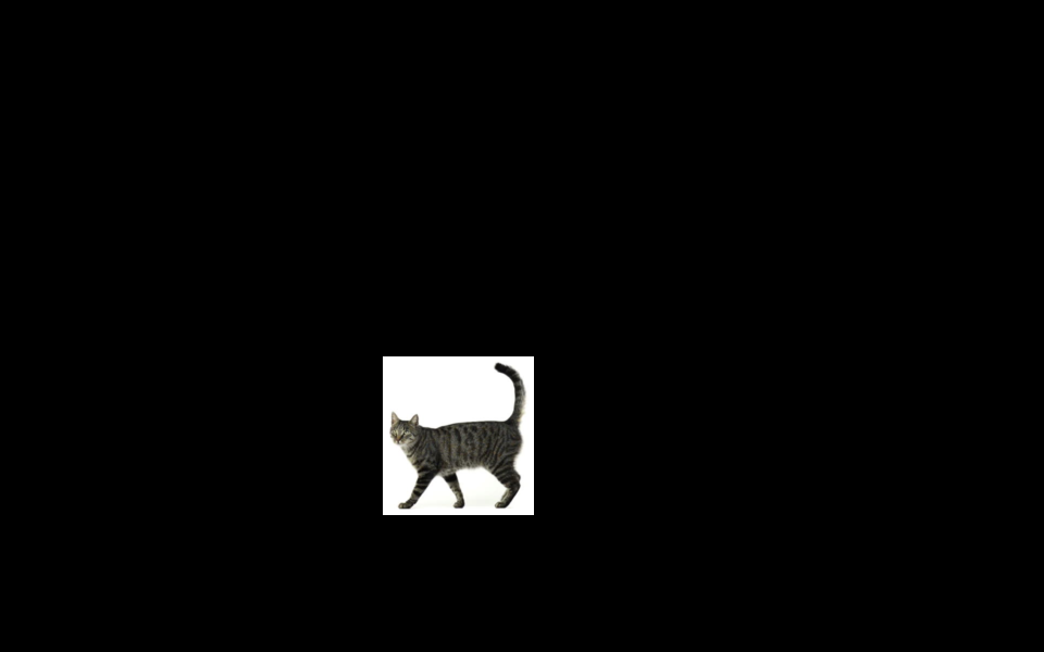 Cat Source Image
|
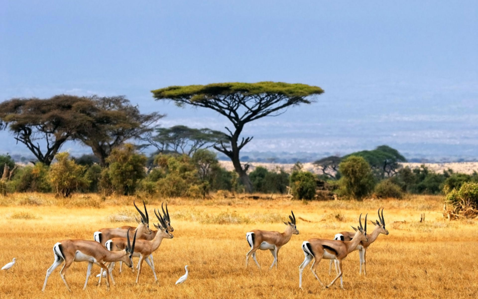 Savannah Target Image
|
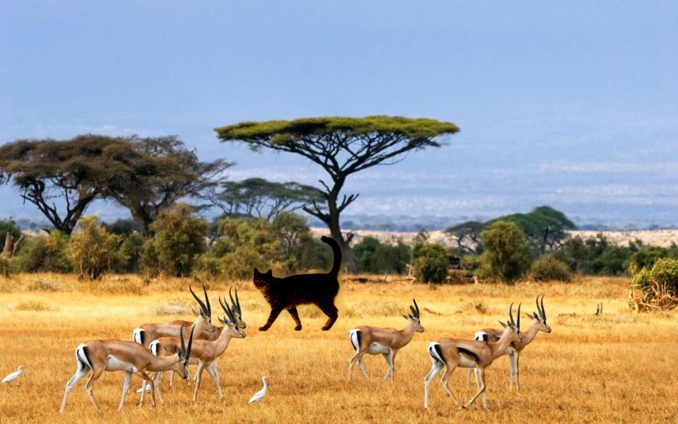 Final Result
|
This poisson blended image of a cat in the savannah resulted in a cat that was overly dark. This result is most likely due to the color difference between the white background in the cat's source image, and the yellow/brown/green background of the savannah target image around the cat. Since poisson blending strives to preserve the gradient of the target image at the edges, it wants to make the white background of the cat source image yellow/brown/green as well. However this color change at the edges of the source image region will propagate throughout the cat source image, causing the cat to turn darker and more yellow/brown/green as well. Since the cat is already fairly dark gray colored to begin with, the propagation of edge gradients causes the cat to turn out too dark in the blended image result.
Laplacian Pyramid Blending vs Poisson Blending
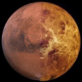
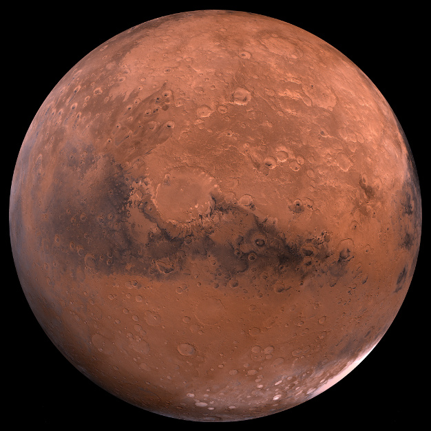 Mars - Original
|
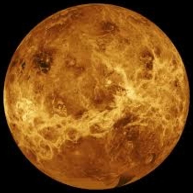 Venus - Original
|
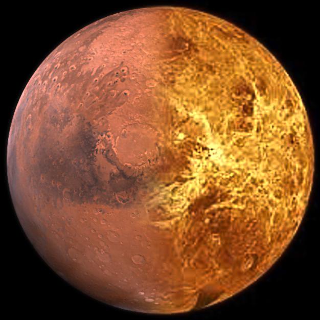 Laplacian Pyramid Blending
|
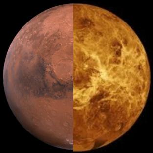 Source Pixels Directly Copied...
|
 Poisson Blending
|
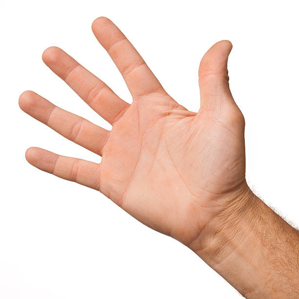
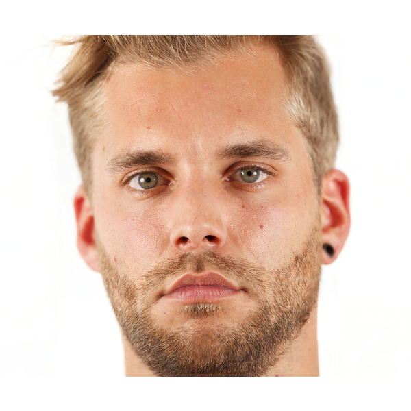
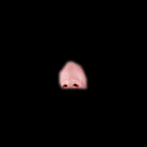
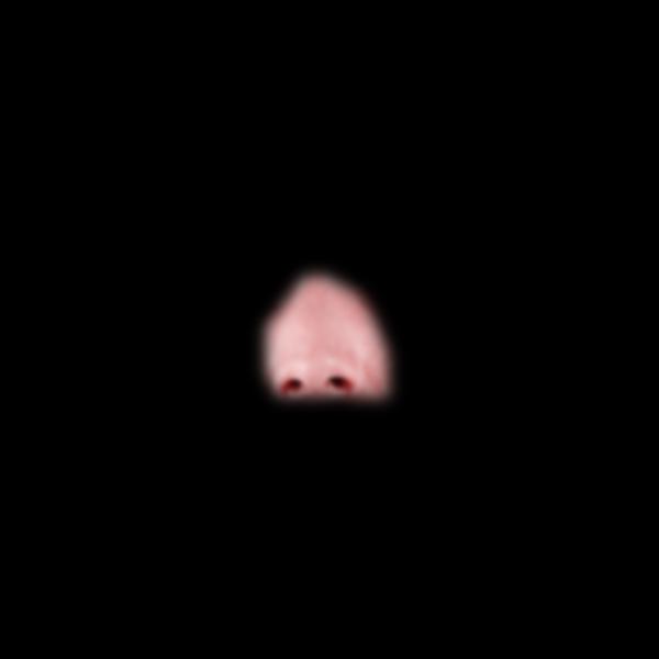
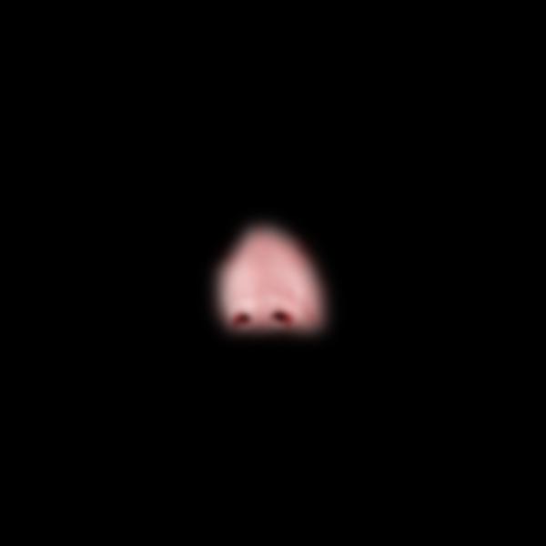
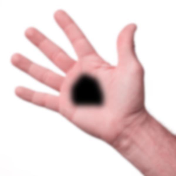
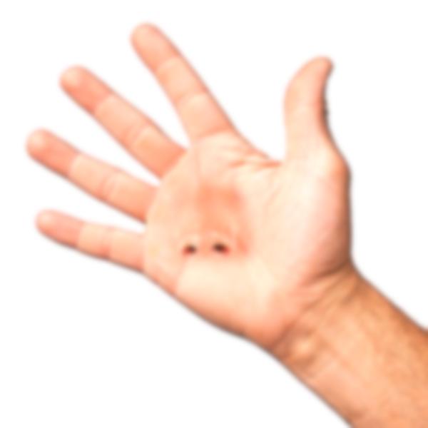
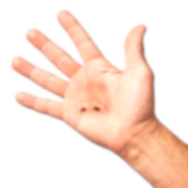
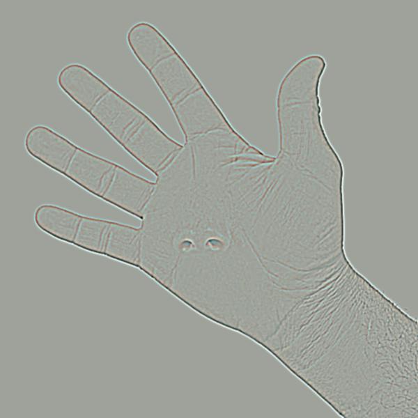
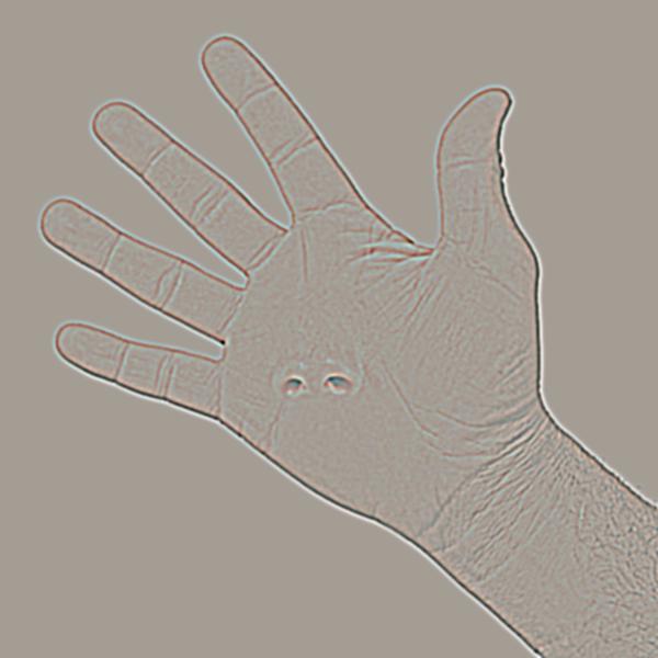
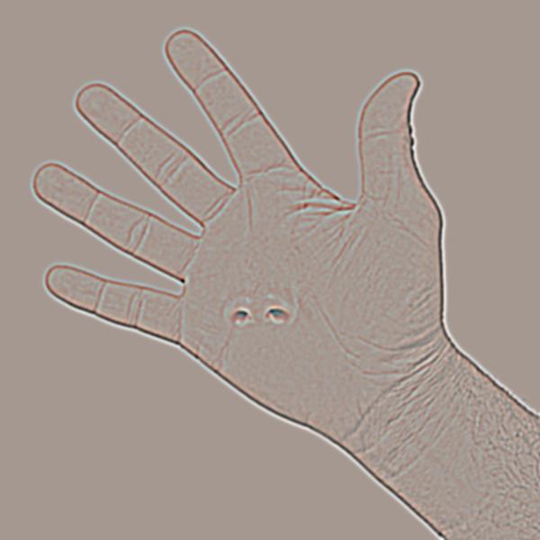
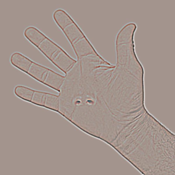
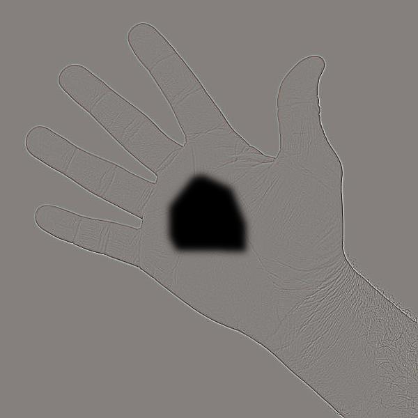
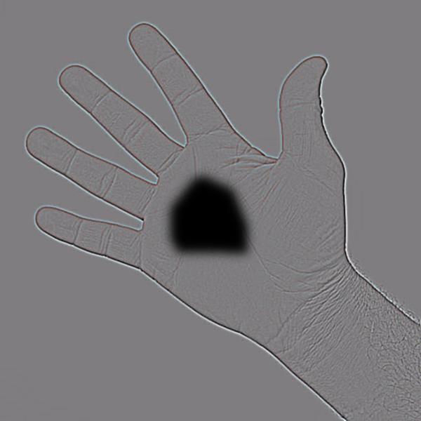
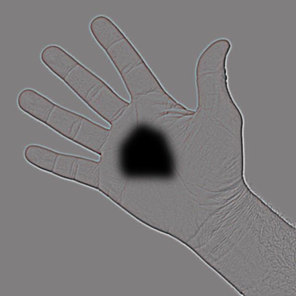
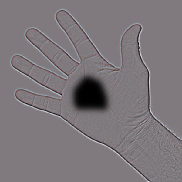
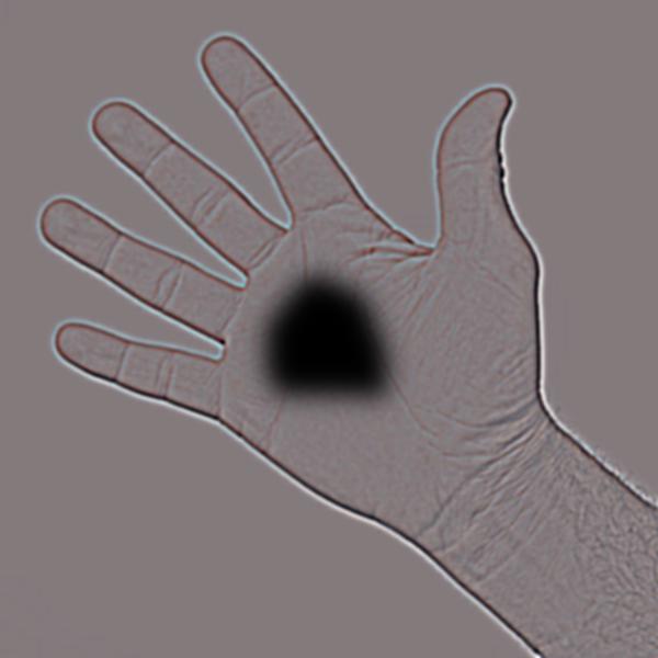
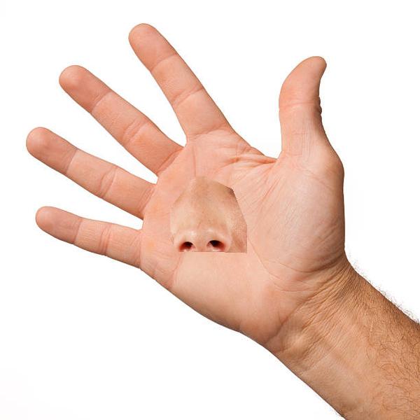
 Hand - Original
|
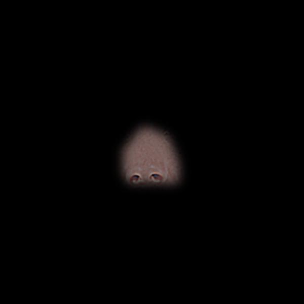
 Face - Original
|
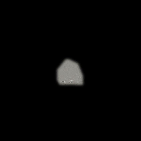
 Laplacian Pyramid Blending
|
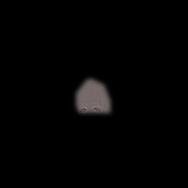
 Source Pixels Directly Copied...
|
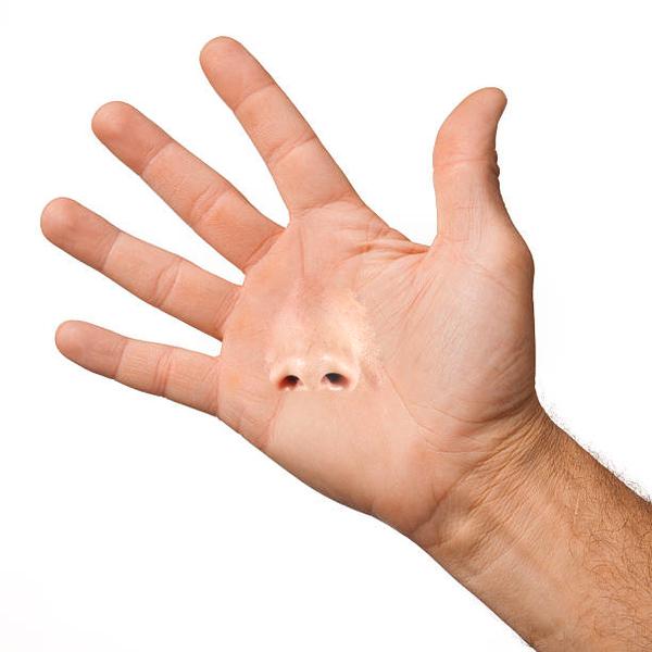 Poisson Blending
|
For the Mars and Venus blend, the poisson blending result was better. Since there is a distinct color difference between Mars and Venus, even though the intensity of the images matched in the laplacian pyramid results, the seam was still very obviously in the middle. Because poisson blending focuses on blending color gradients, the resulting blended image was smoother overall in terms of color, and had a less obvious seam. I feel like the hand and nose blended image also had a better result with poisson blending. While the edges are smoother in the laplacian pyramid result, the color of the nose is noticably darker and redder than that of the hand, causing it to stand out. Meanwhile, with poisson blending, while the edges are less smooth due to differences in intensity between the source and target image, the color of the hand and the nose is closer, and hence feels better blended.
As we can see with the cat in savannah example for poisson blending, and the Mars and Venus example for laplacian pyramid blending, laplacian pyramid blending can result in very noticable seams if there are color differences, and poisson blending can greatly alter the color of a source image. As a whole, if we value obtaining image seams that are smoother in intensity, laplacian pyramid blending is the better choice. On the other hand, if blending and smoothing out an image's gradient is more valued, then poisson blending is the better choice.
Important Things Learned
The most important thing I learned from this project are the theories and steps behind implementing laplacian pyramid blending and poisson blending, as well as the tradeoffs for when to use each blending technique.