Part 1.1 Warmup
To sharpen an image, I took the original image and subtracted the gaussian to produce a detailed image. Then, I added the detailed image (multiplied by a constant) back onto the original image to achieve a sharper image.
original + blurred

detailed + sharpened
Part 1.2 Hybrid Images
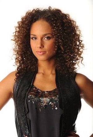
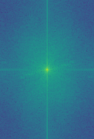
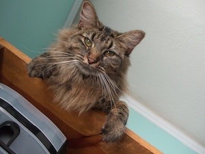
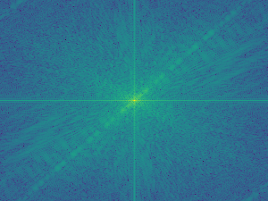
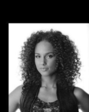
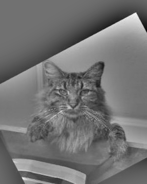
To create a hybrid image of both high and low frequencies, the images first had to be aligned. After alignment, we applied a guassian to the image we want to see further away (Alicia Keys). For the image we want to see upclose (Nutmeg), we apply a high pass filter to obtain the image's high frequencies. As a result, we get a hybrid image when we add the low frequencies of Alicia Keys and the high frequencies of Netmeg together.
alica_keys + alicia_keys_fft
nutmeg + nutmeg_fft
blurred_alicia_keys + sharp_nutmeg
nutmeg_and_keys

Additional Results
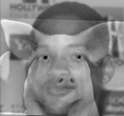
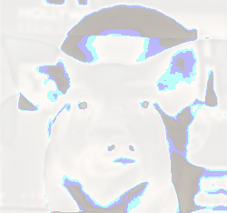
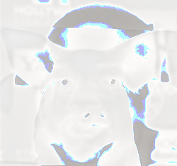
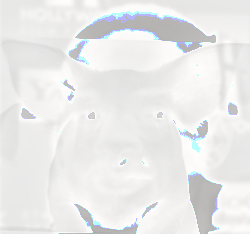
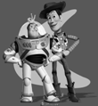
piggy_and_will_smith
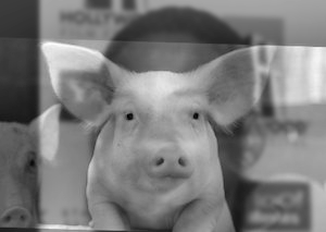
Although the eyes were able to align properly, we can see the piglet's snout does not blend well with Will Smith's nose and mouth.
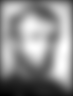
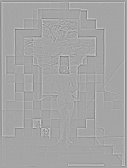
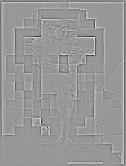
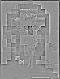
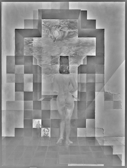
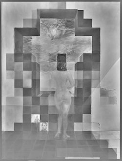
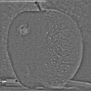
Part 1.3 Gaussian and Laplacian Stacks
Here we apply gaussian and laplacian filters to enhance the visual effects of the hybrid images. As the image gets blurrier, lower frequencies are more visible. On the other end as the image gets sharper, higher frequencies become more apparent.
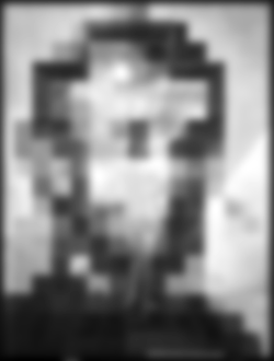
grey_lincoln.jpg

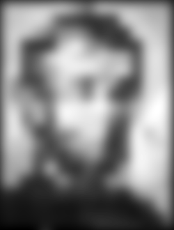
sharp_lincoln.jpg
piggy_and_will_smith.jpg
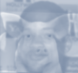


sharp_piggy_and_will_smith.jpg
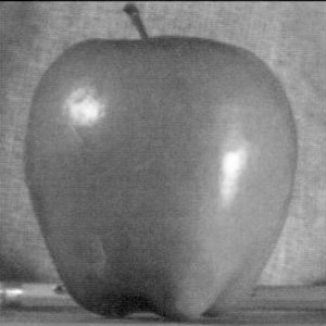
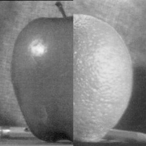
Part 1.4 Multiresolution Blending
Here we attempt to blend two images together seamlessly. Although the blend looks okay in the detailed version, the blended image without any filters can be improved.
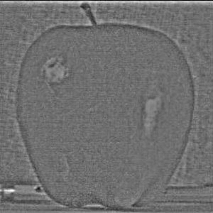
apple
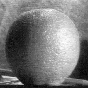
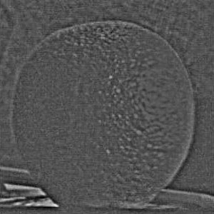
orange
orapple
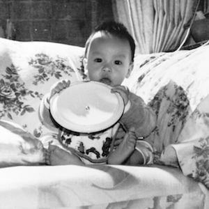
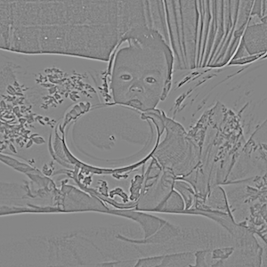
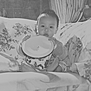
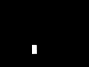
Part 2.1 Toy Problem
In this section, we compute the x and y gradients of an image to solve an least squares objective function. Formulating this in psuedocode, we create a (2(mn)+1 x mn) matrix A to hold our x and y gradients of an (mxn) image. An addtional row is added to ensure that the top left corner of the reconstructed image will have the color as that of the original image. We create a (2(mn)+1 x 1) vector B which consists of the gradient values of the original image. Solving the equation Av = b for v, we reconstruct the original image.
original + reconstructed

Part 2.2 Poisson Blending
To poisson blend a source object image onto a target background image, we extend our idea from part 2.1. Using the starter matlab code, we first select a region in the source image and then a location that we would like to blend into our target background image. Afterwards, we align the source image so that the mask corresponds to the location in the target image.
Using the mask, we can determine a border around the object we are trying to blend into the background. With an equation for each border pixel, we add these rows to our matrix A so that we can get the pixel intensities around the object border that closely matches the background pixels.
Solving for the v values, we can replace the pixels in our background image to achieve a poisson blended image.
Source + Border + Mask + Target

Poisson Blending