Fun with Frequencies and Gradients
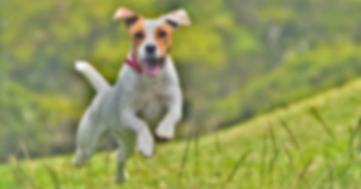
The objective of this part was to take a blurry image and sharpen it using the unsharp masking technique. I got a highpass filter of the image by subtracting the Gaussian filter (with sigma = 25) from the original image. This filter is then multiplied by some weight (alpha) and added on to the original image.
Original Image
alpha = 0.5

alpha = 1
alpha = 2
alpha = 10
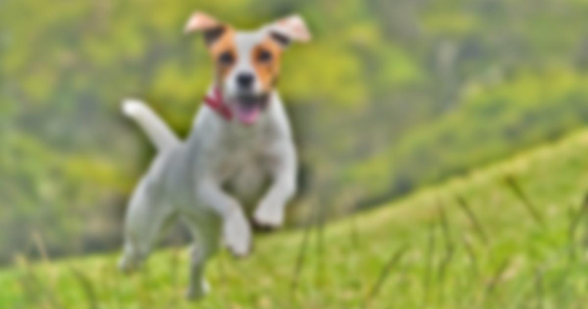
alpha = 100
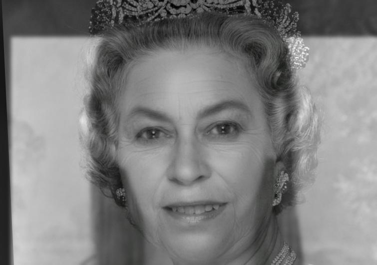
The objective of this part is to create a hybrid image from two images such that one image appears when looking at it from up close and another appears from far away. This is accomplished by adding together the highpass filter from one image and the lowpass filter of another image. The frequency cutoffs for each filter were chosen empirically.
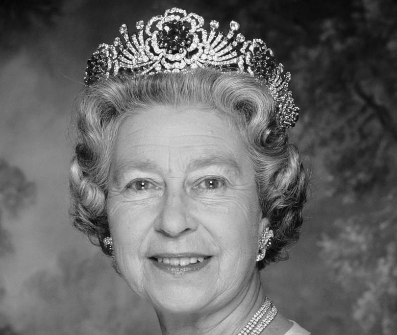
Queen Elizabeth II
Highpass filter (sigma = 32)
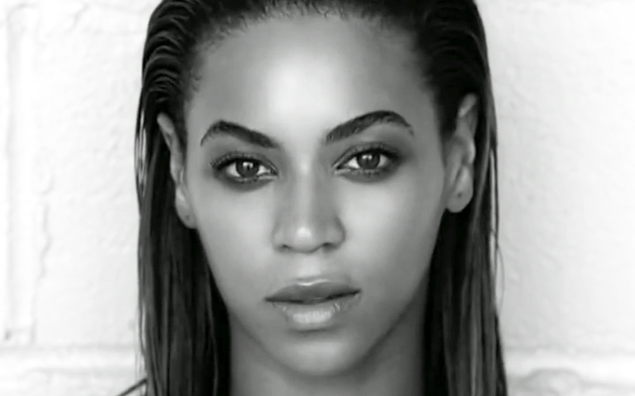
Beyonce
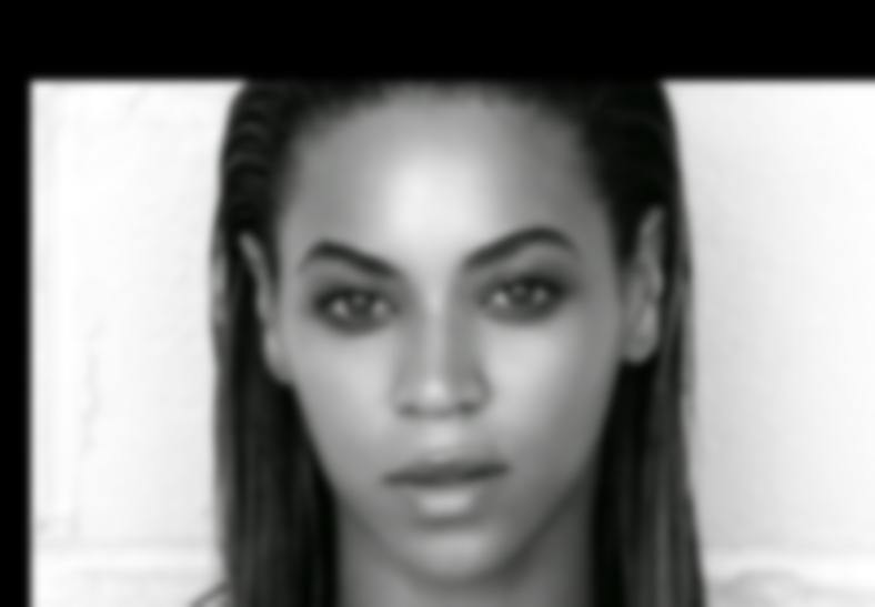
Lowpass filter (sigma = 4)
Queens
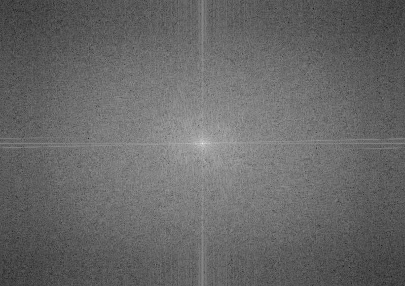
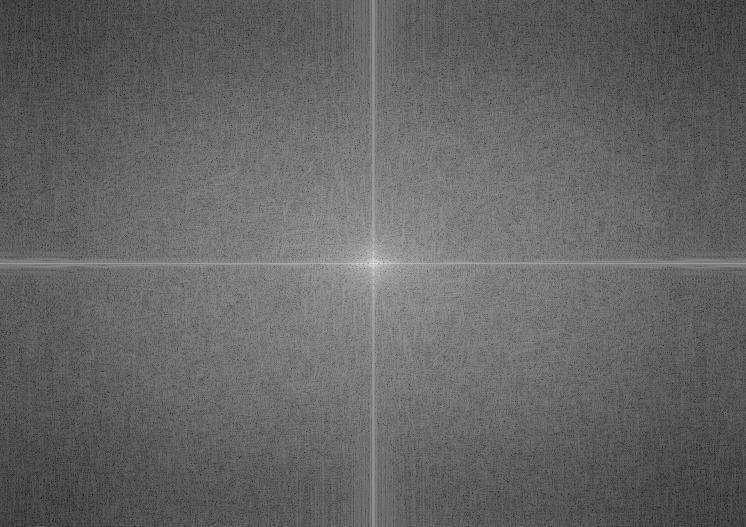
The FFT Analysis of the above images are as follows:
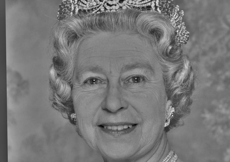
Aligned Image Queen
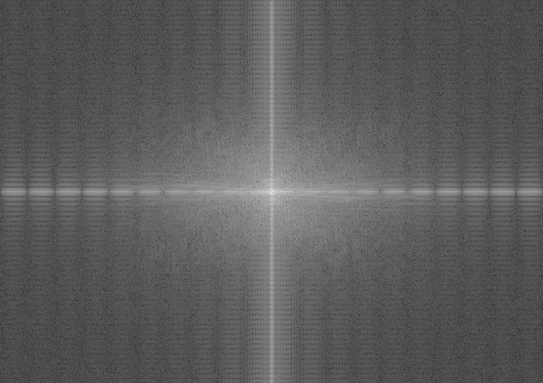
Aligned Image Beyonce
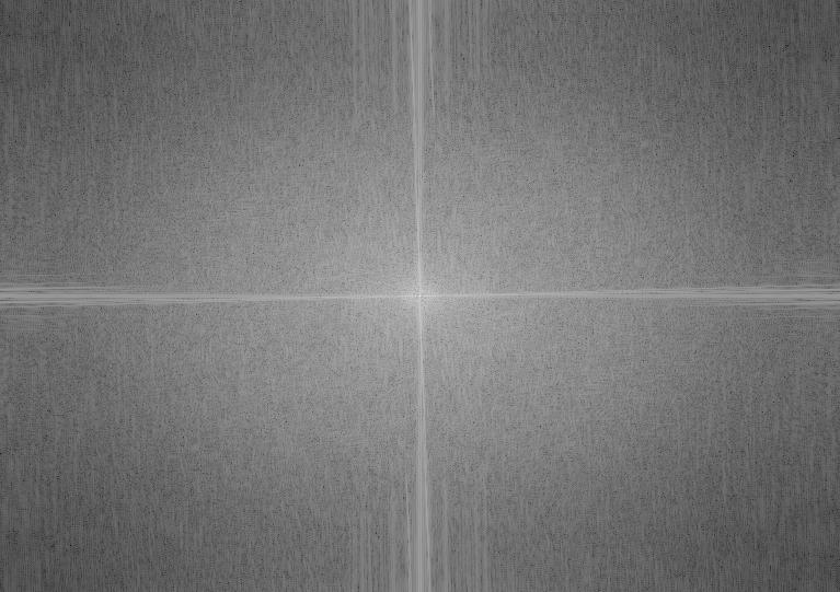
High Frequency Queen
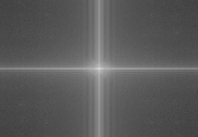
Low Frequency Beyonce
Hybrid Image
Here are a couple additional hybrid images:
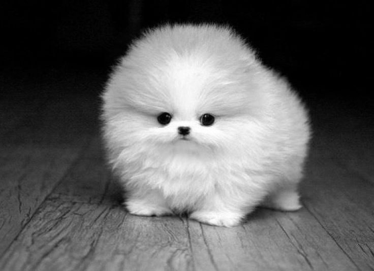
Baby Animal 1 (Highpass sigma = 64)
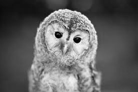
Baby Animal 2 (Lowpass sigma = 4)
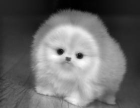
Baby Animals
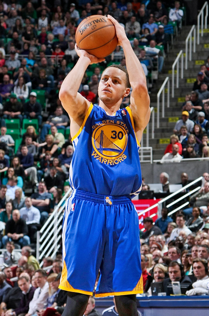
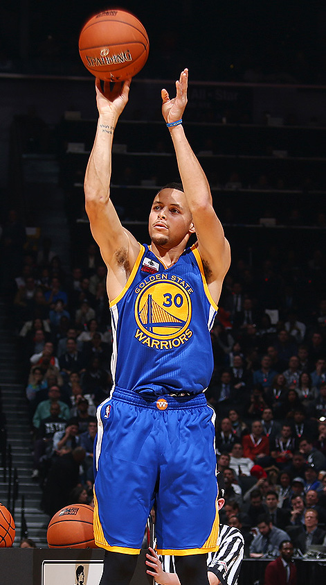
Steph Curry 1 (Highpass sigma = 128)
Steph Curry 2 (Lowpass sigma = 4)
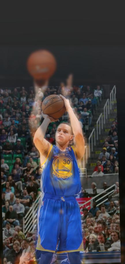
Steph Curry Shooting
The baby animals and Steph Curry ones did not turn out as nicely as the other ones did. A big reason for that was that the images did not line up very well.
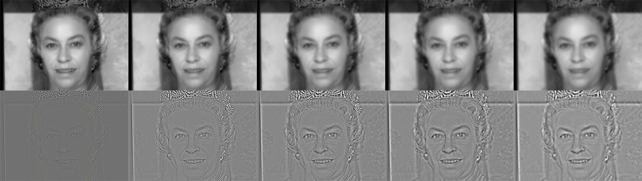
The objective of this part was to implement Gaussian and Laplacian Stacks. The Gaussian stack of each image is computed by repeatedly applying a Gaussian filter (of increasing sigma) at each level. This differs from a pyramid in that the size of the image is preserved, but the image becomes more and more blurred as you go down the stack. The Laplacian stack is calculated by taking the difference between each level of the Gaussian stack and the next level.
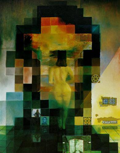
Original Image
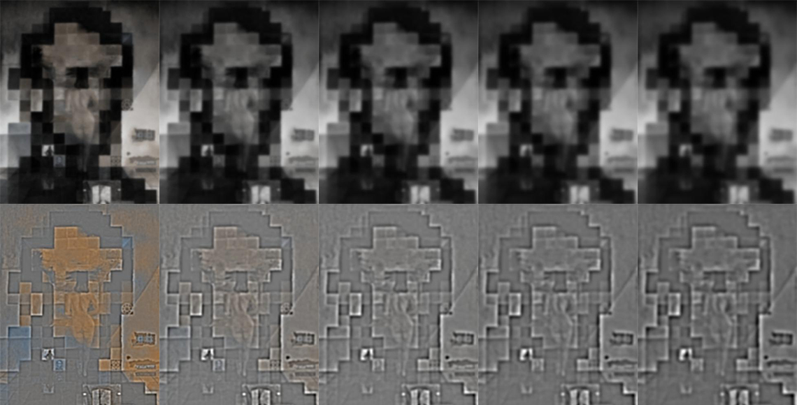
Gaussian Stack (top) and Laplacian Stack (bottom)
sigma = 2, 4, 8, 16, 32
Original Image
Gaussian Stack (top) and Laplacian Stack (bottom)
sigma = 2, 4, 8, 16, 32
For this part, we are using the Gaussian and Laplacian stacks from the previous part to blend together two images seamlessly. To do this, we create Gaussian and Laplacian stacks for both of the images, and a Gaussian stack for a mask image. For example, we are using a vertical seam for the oraple, so the mask image simply consists of 1's on the left and 0's on the right (or vice versa). At each level of the stack, we apply the equation below to obtain the resulting image of that level:

Now we just have to sum up the levels and add in the last level of each image's Gaussian stacks, weighted properly.
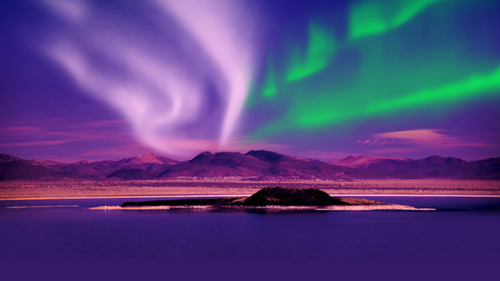
Northern Lights
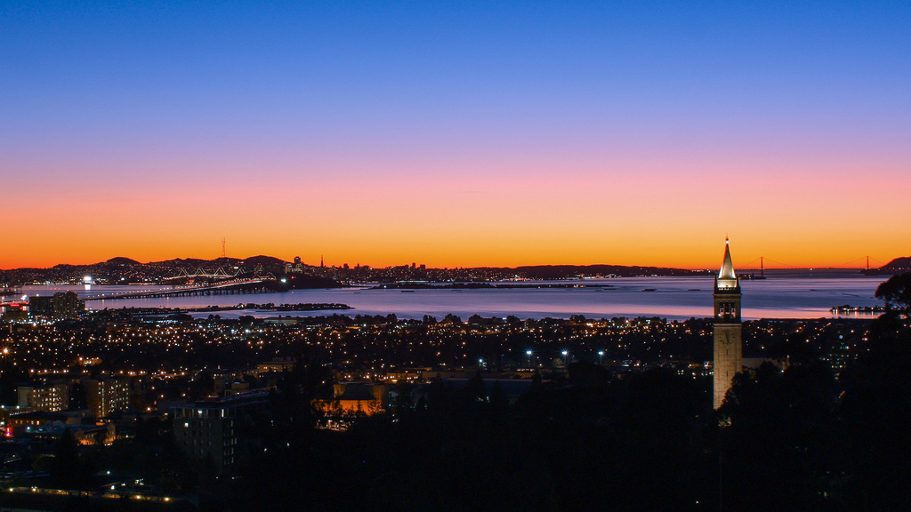
Berkeley

Horizontal Mask
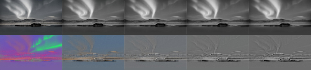
Northern Lights Gaussian and Laplacian Stacks (same format as above)
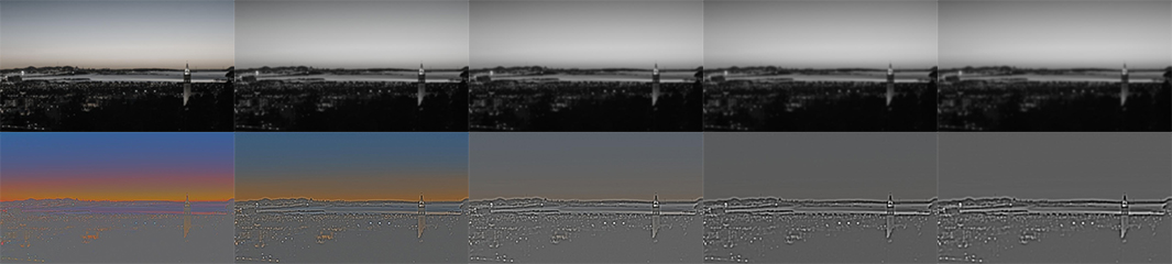
Berkeley Gaussian and Laplacian Stacks (same format as above)
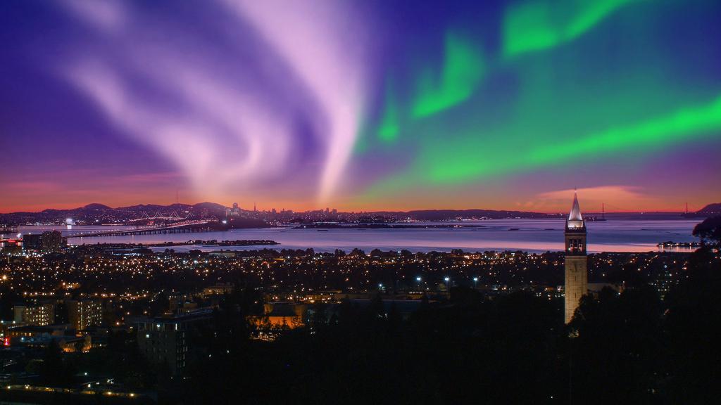
Northern Lights over Berkeley
Here are some additional examples:

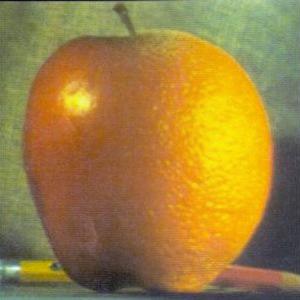
Apple

Orange

Vertical Mask
Oraple
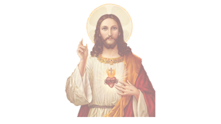
Jesus
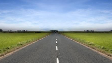
Road
Horizontal
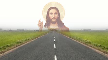
Highway to Heaven
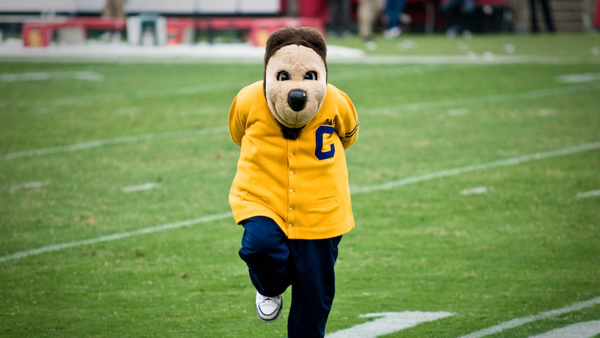
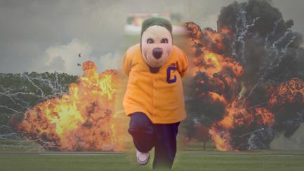
Oski
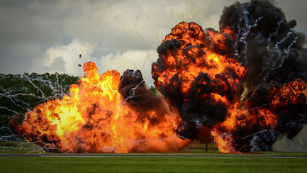
Explosion
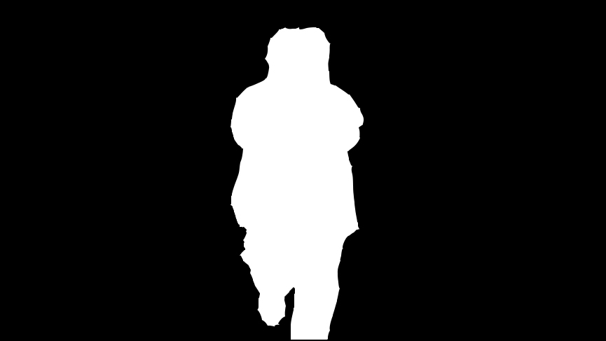
Custom Mask
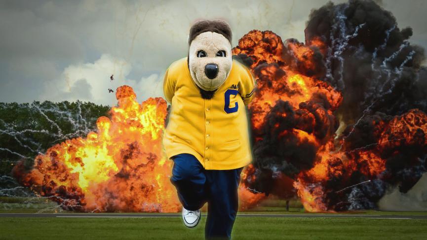
Oskiplosion
To account for color, we process each color channel separately. We first separate the color channels and apply the above method to the 2-dimensional image. We then stack the results together to get back a color image.
This part of the project uses gradient domain processing to blend together images. The goal is to seamlessly blend together two images using a technique called "Poisson Blending." We do this by formulating this as a least squares problem, and minimizing the gradient differences between the source and target images.
For the toy problem, we are trying to reconstruct an image using this technique. For an image that's h x w, we have 2 * h * w + 1 constraints: we want to minimize the gradient between each pixel and its neighbor to the right, each pixel and its neighbor below, and the gradient between the top left corner of the new image and the original image.
Here are the results of the reconstructed image:
Original Image

Reconstructed Image
Now we blend together our source and target images using the following set of constraints:

We first select the region in our source image we want to copy over. Then, for each color channel, we solve our least squares problem of minimizing the gradient at the seam of the two images. Once we find the pixel values that minimize the gradient, we copy those over to the appropriate place in the target image. Lastly, we stack together the color channels to form our final output image.
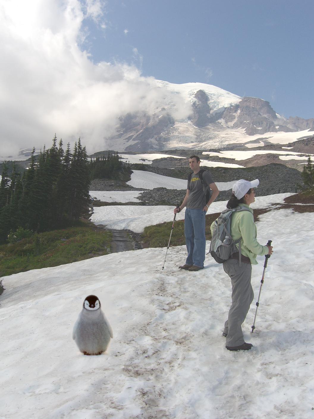
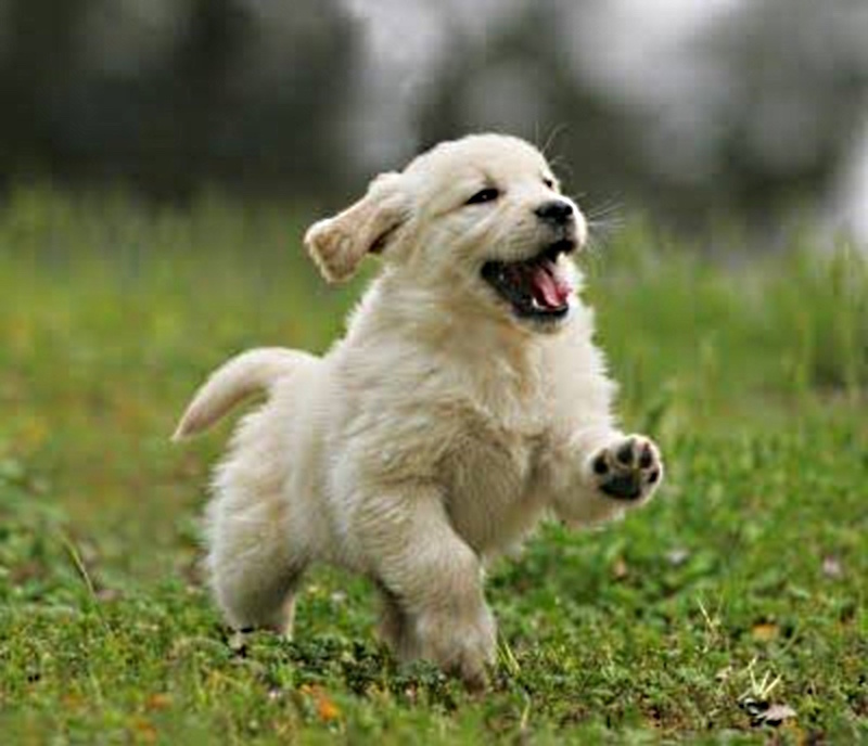
Source Image
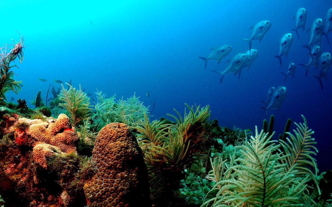
Target Image
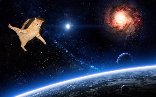
Directly Copied Over Image
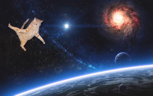
Poisson Blended Image
Here are some additional examples of Poisson blending:
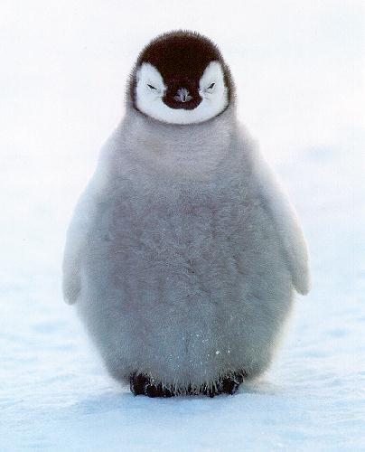
Source Image
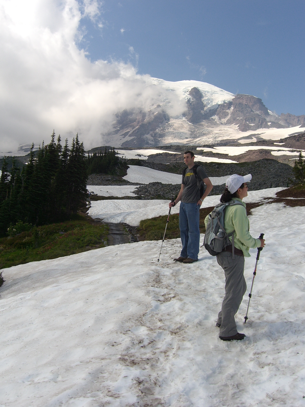
Target Image
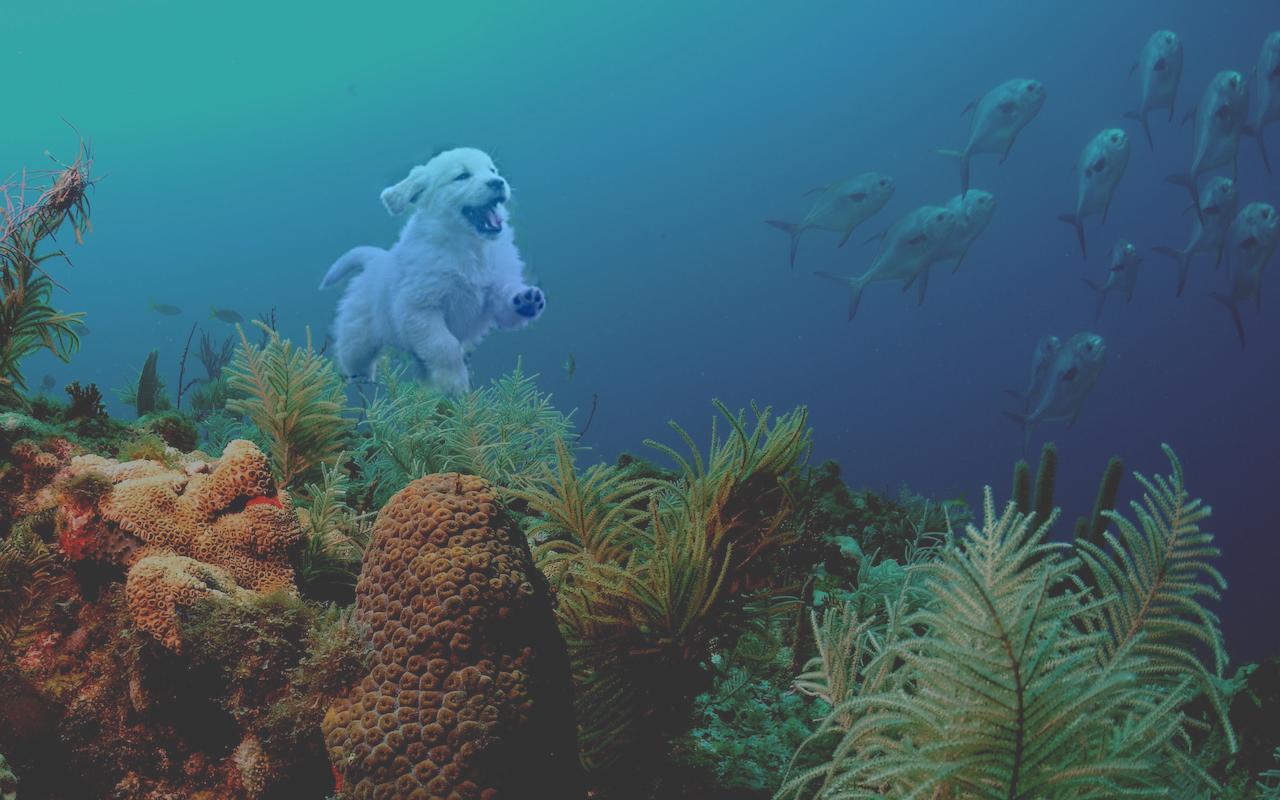
Poisson Blended Image
Source Image
Target Image
Poisson Blended Image
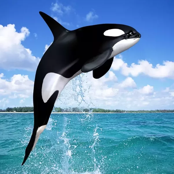
Source Image
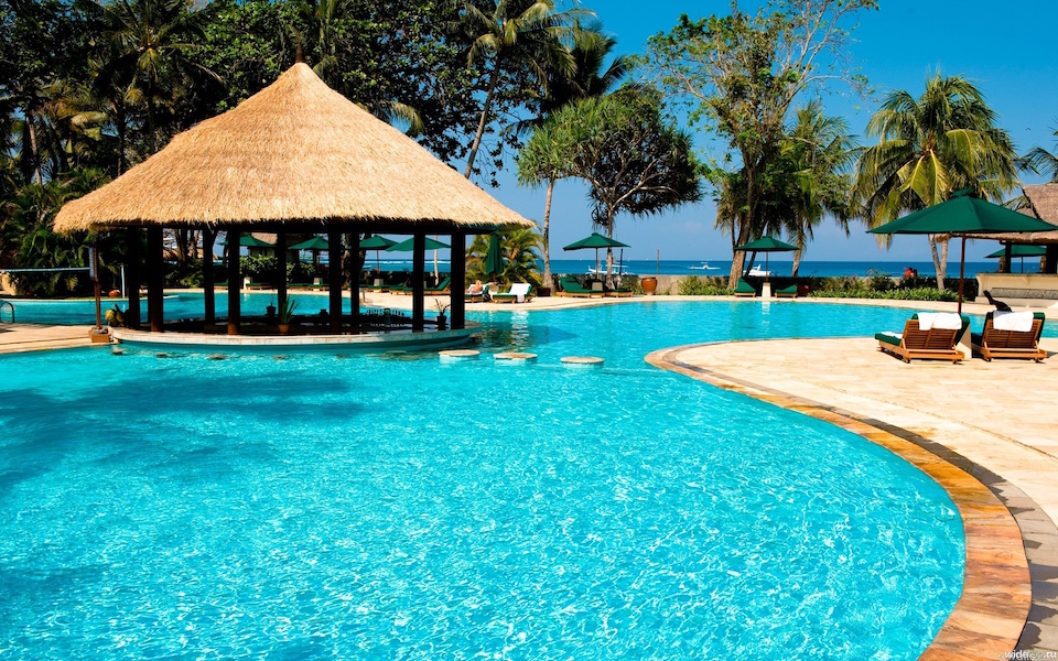
Target Image
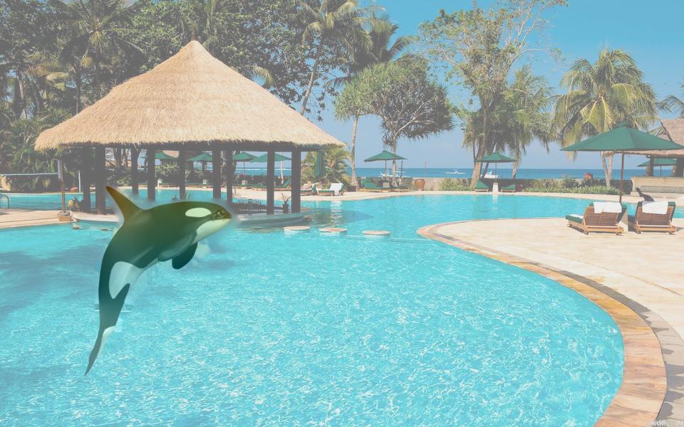
Poisson Blended Image
Source Image
Target Image
Poisson Blended Image
The Poisson Blended image of Oskiplosion was not as good as the one blended with Laplacian stacks. This could be because the differences between the two colors at the seam are too obvious, so even blended, we can see a bit of a seam. The coloring for the dog underwater is also a little off, as gradient domain fusion does not deal as well with maintaining original colors.