CS 194-26: Project 3

Fun with Frequencies and Gradients

Ellen Hong

Overview

In this project, we explore the applications of the frequency and gradient domains in the context of image manipulation, including how to sharpen images and blend them together seamlessly.

Part 1: The Frequency Domain

Part 1.1 (Warm-up): Unsharp Masking

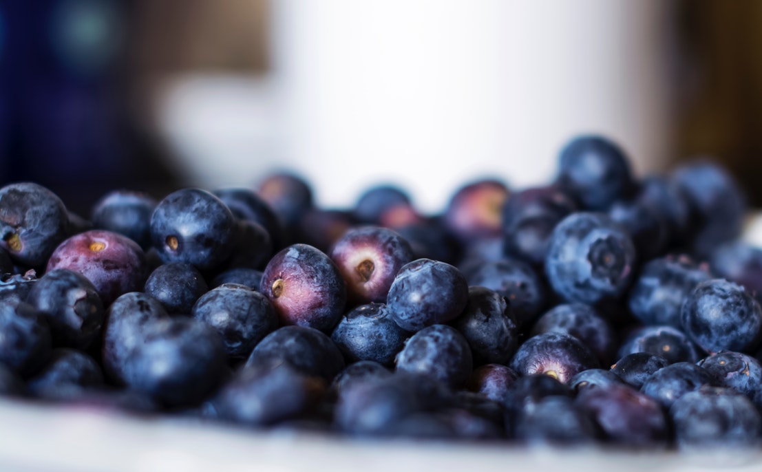
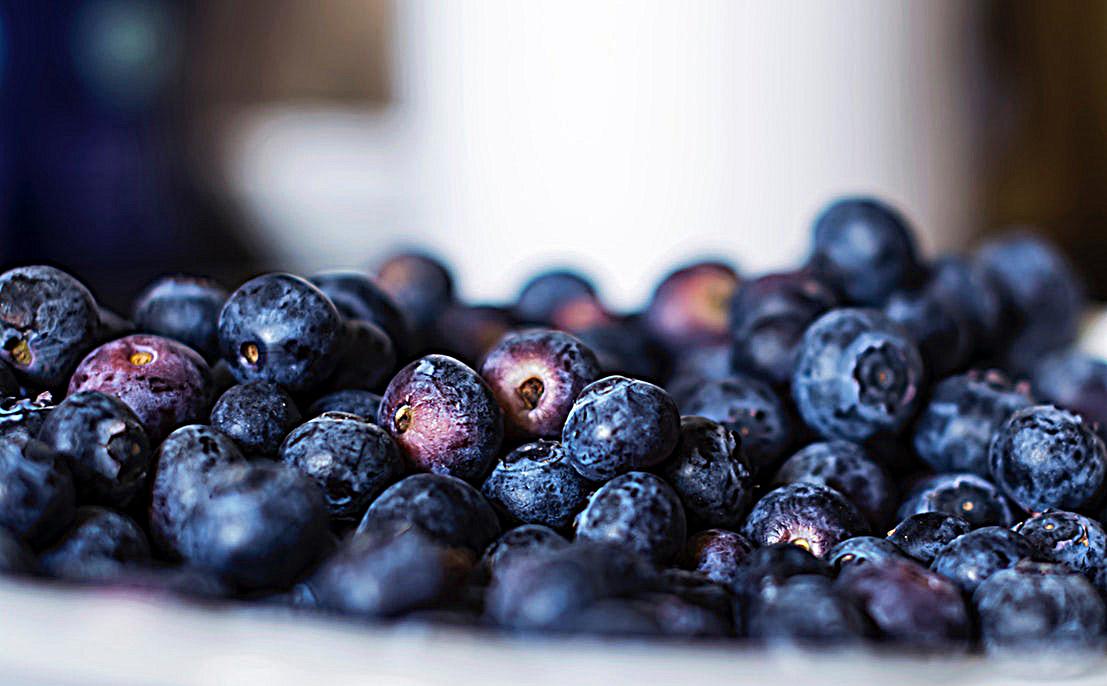
In this warm-up exercise, we implement the unsharp masking technique: we first obtain the low frequencies of the image by applying a Gaussian filter, then extract the high frequencies by subtracting the Gaussian blurred image from the original. We add these high frequencies back to the original image to obtain a sharpened image.

Part 1.2: Hybrid Images

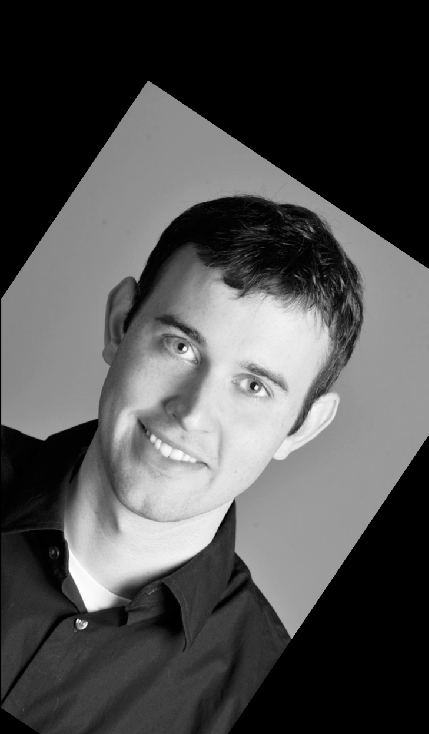
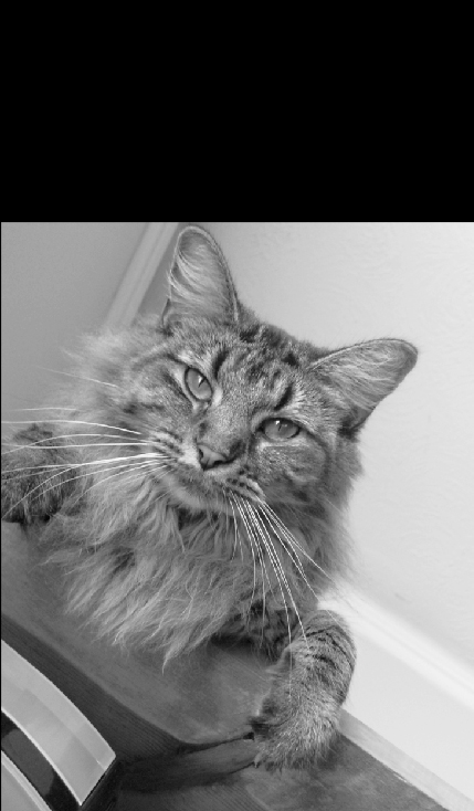
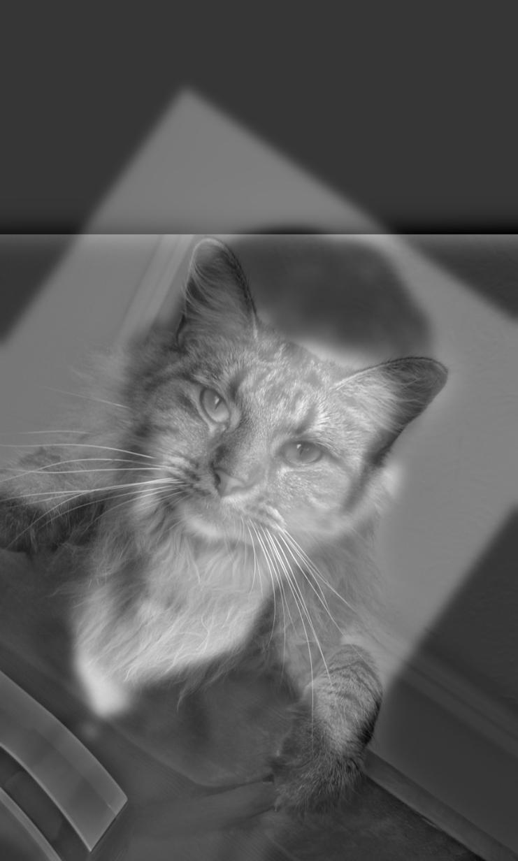
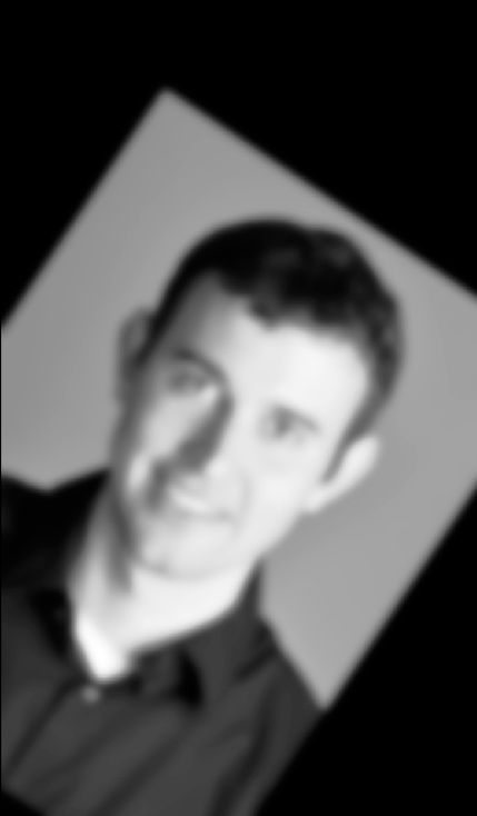
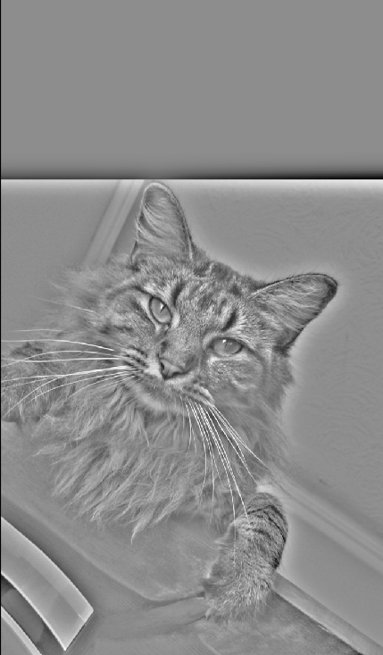
The way we perceive images can differ drastically in different frequency domains. We can take advantage of this fact in creating hybrid images: images that will reveal high frequencies of one image at shorter distances, and low frequencies of a different images at longer distances. Thus, the method implemented below is to, after aligning the images, low-pass filter one & high-pass filter the other, then add them together. We see the results below from blending together Derek and his cat Nutmeg.

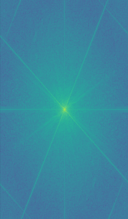
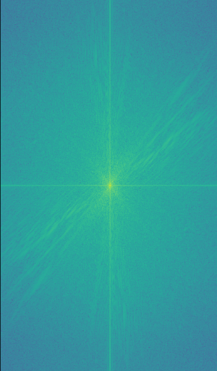
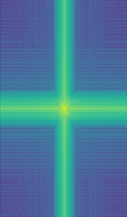
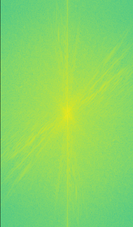
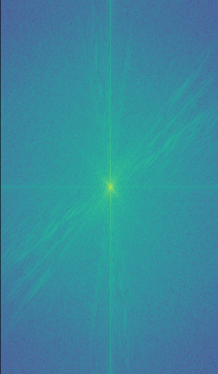
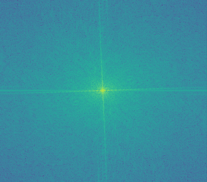
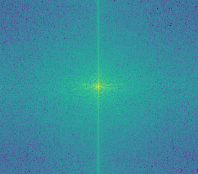
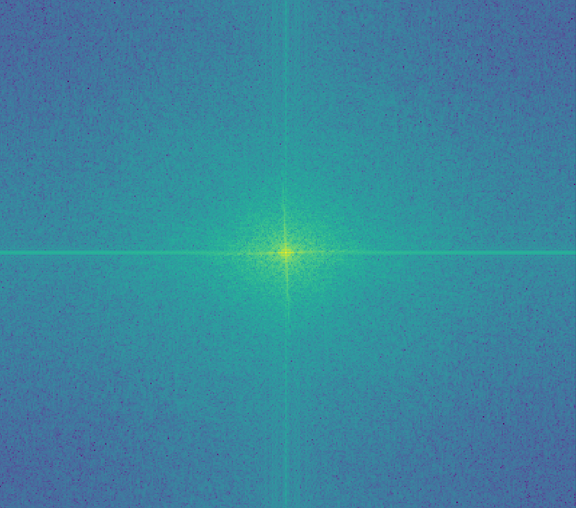
We can also perform a frequency analysis on these images to get a better understanding of how the frequencies look at each stage of the process. Shown below are the log magnitudes of Fourier transforms of the input images.

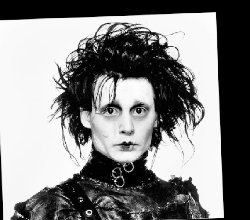
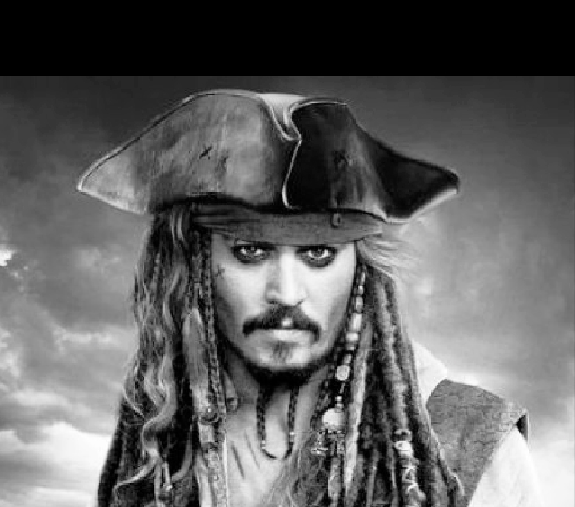
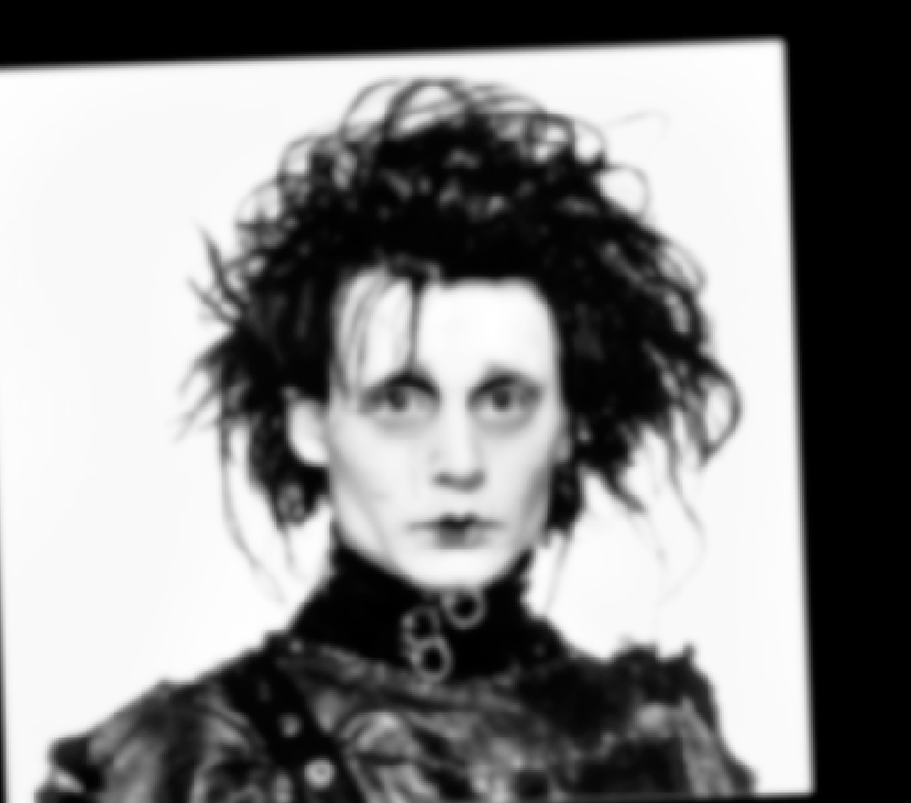
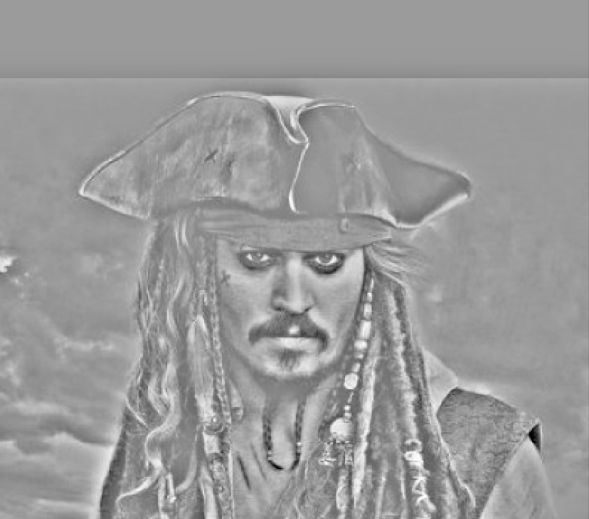
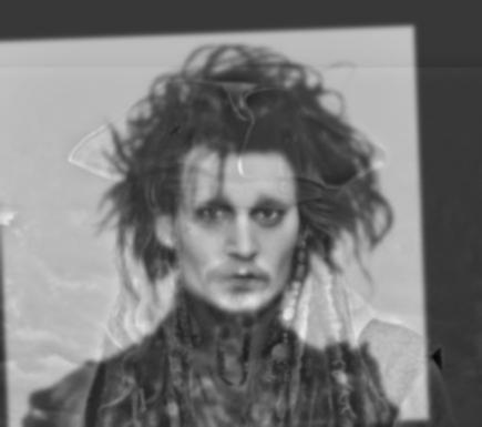
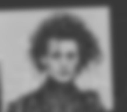
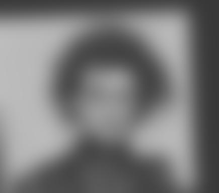
Second set of results: Hybrid of Edward Scissorhands and Jack Sparrow (both played by Johnny Depp).

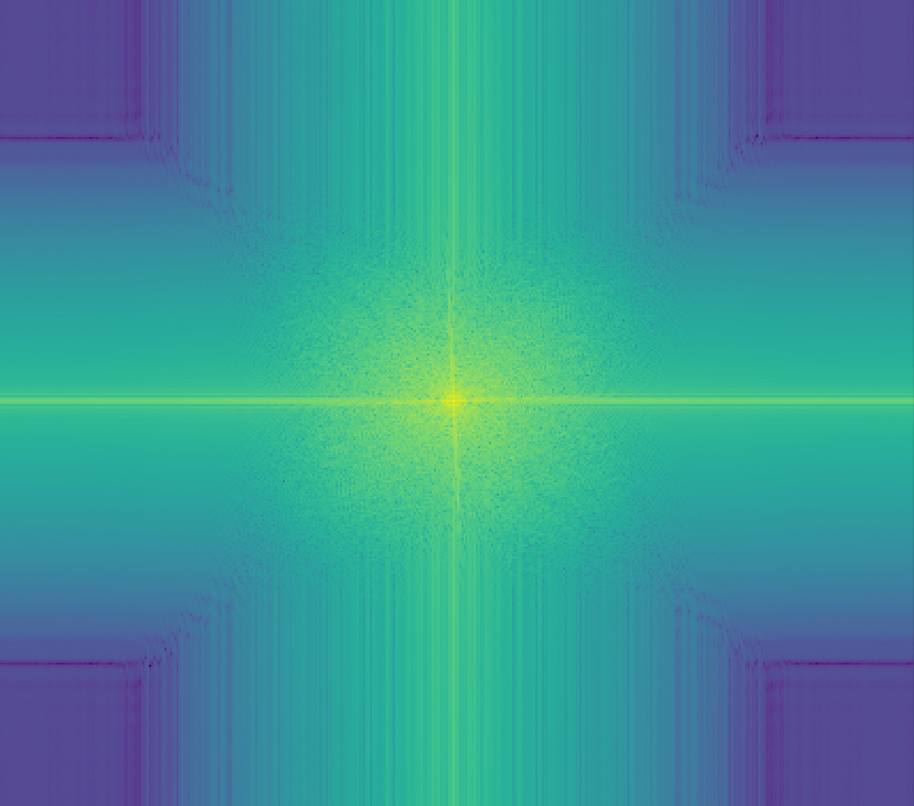
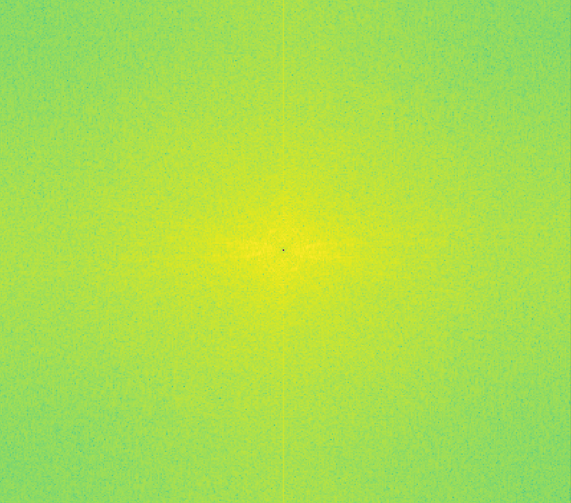
Again, we show the various log magnitudes of Fourier transforms of the input images.

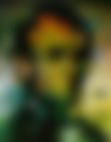
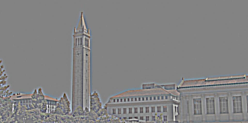
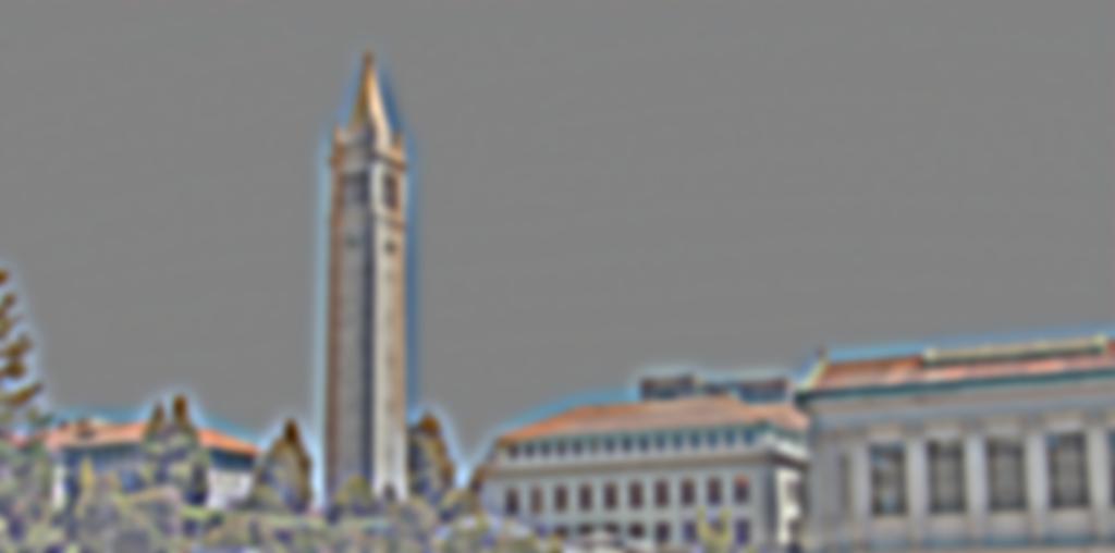
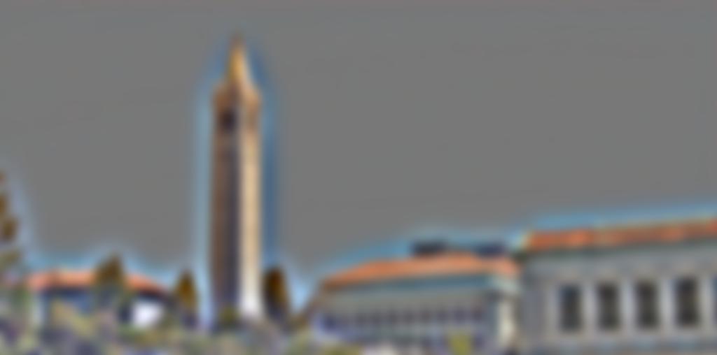
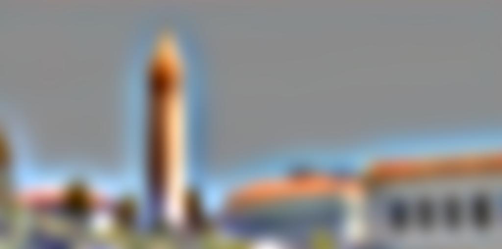
Part 1.3: Gaussian and Laplacian Stacks

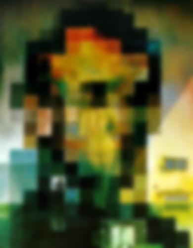
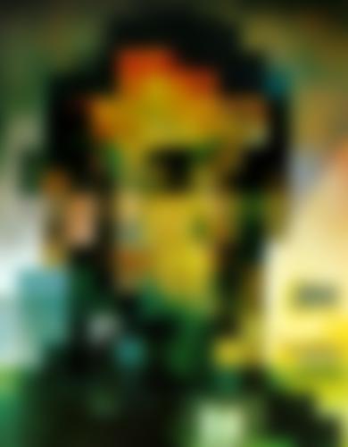
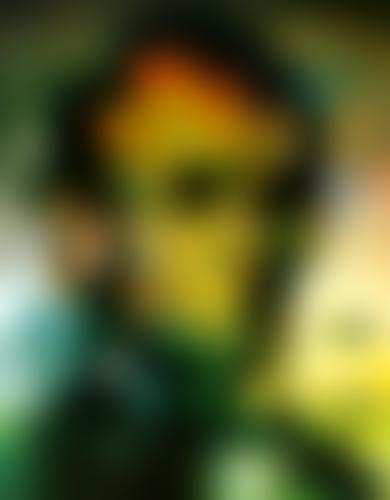
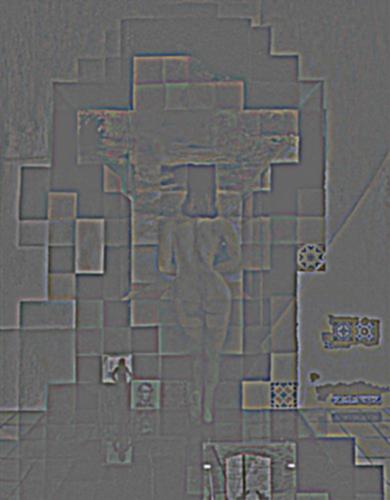
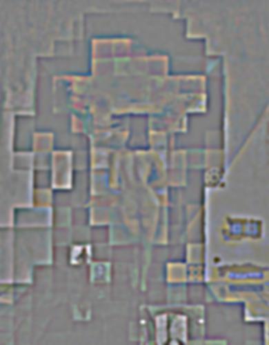
We further explore the frequency domain by creating Gaussian and Laplacian stacks. A Gaussian stack is created by applying a Gaussian filiter to the input image, then repeatedly applying Gaussian filters with higher sigma values at each level. The corresponding Laplacian stack is created by taking differences between consecutive images in the Gaussian stack. We visualize the results on the Salvador Dali image below.

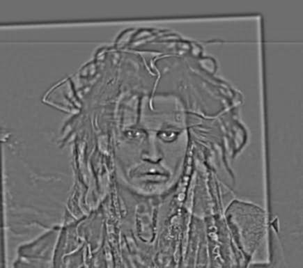
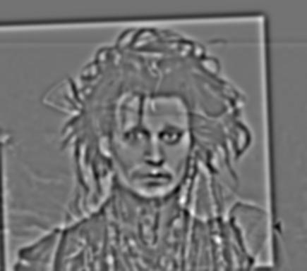
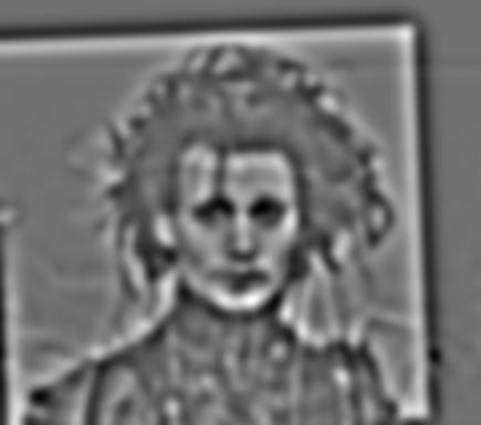
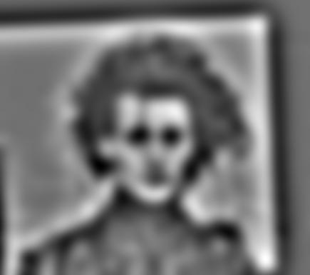
We also create Gaussian and Laplacian stacks for our hybrid of Edward Scissorhands and Jack Sparrow. Notice that doing so reveals the individual components of the hybrid.

Part 1.4: Multiresolution Blending

We now explore multiresolution blending, which is a technique that takes two images and creates a seamless blend between them. The method we use, in this case, is the masking method described in this paper:

For input images A and B, we construct Laplacian stacks LA and LB for each image. We then construct a Gaussian stack for the mask, and form a combined pyramid according to the following equation:
LS_l(i, j) = GR_i(i, j)LA_l(i, j) + (1 - GR_l(i, j))LB_l(i, j)

Essentially we use the nodes of mask's Gaussian stacks as weights for Laplacian pyramid LA, and the inverse of those nodes as weights for Laplacina pyramid LB. Adding these levels creates a Poisson blended result.

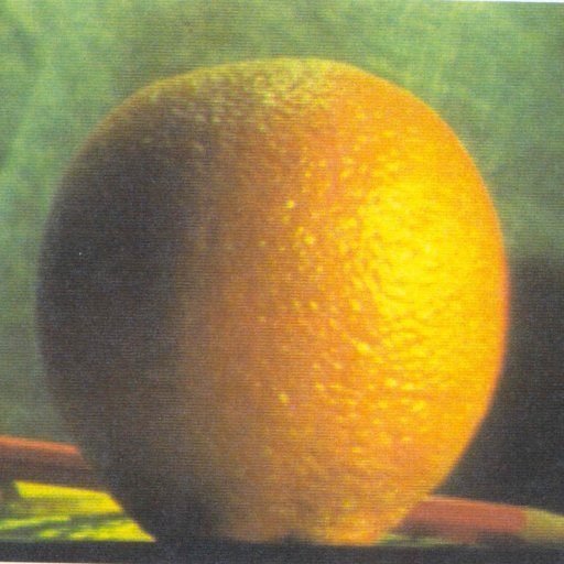
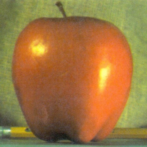
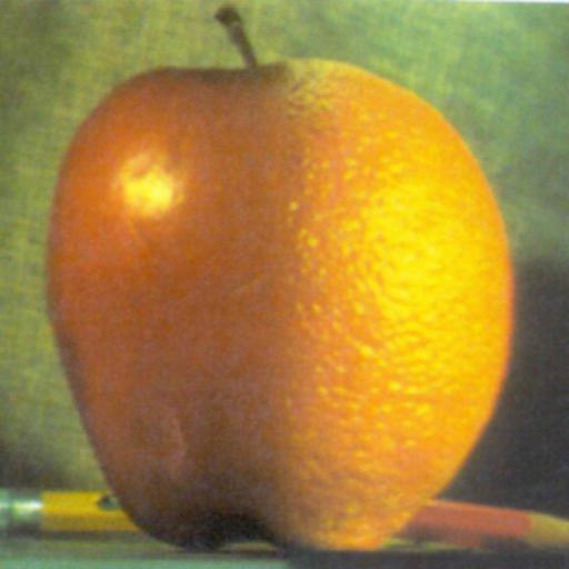
Below are the results of the sample images, the orange and the apple, blended together.

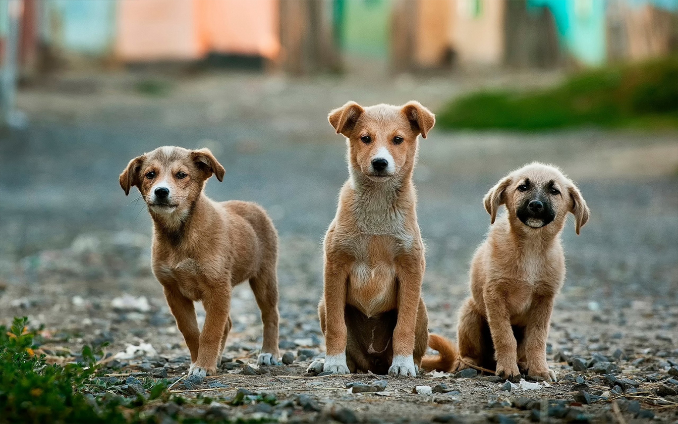
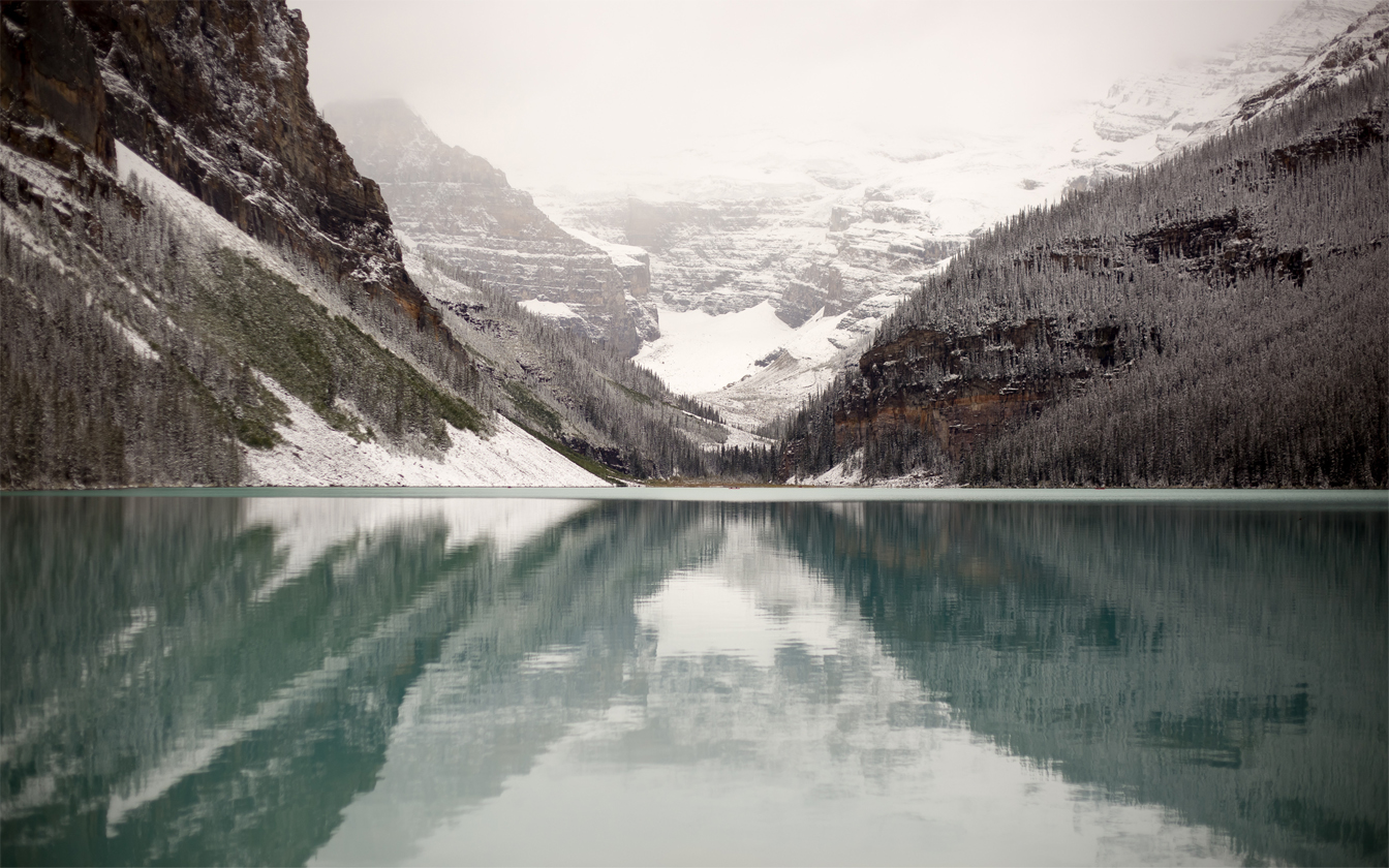
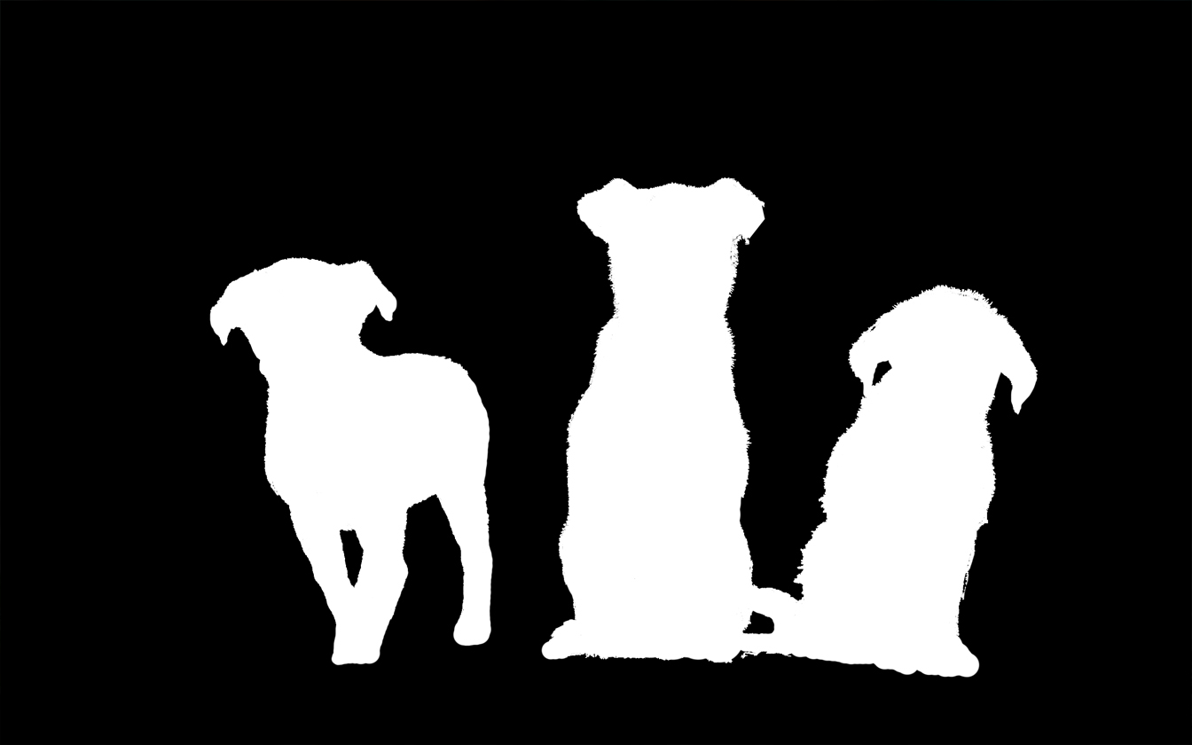
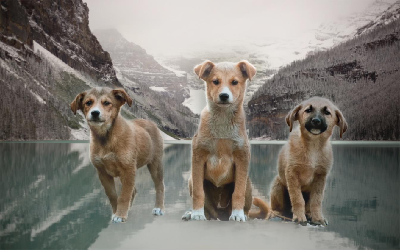
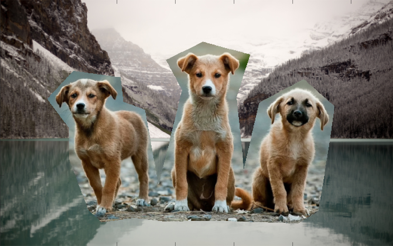
We attempt to place a dogs into a mountain/lake backdrop.

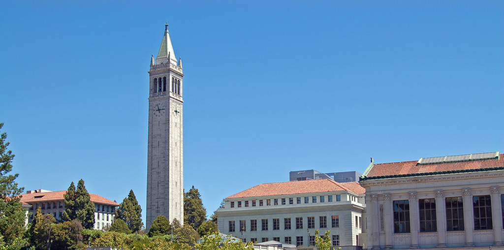
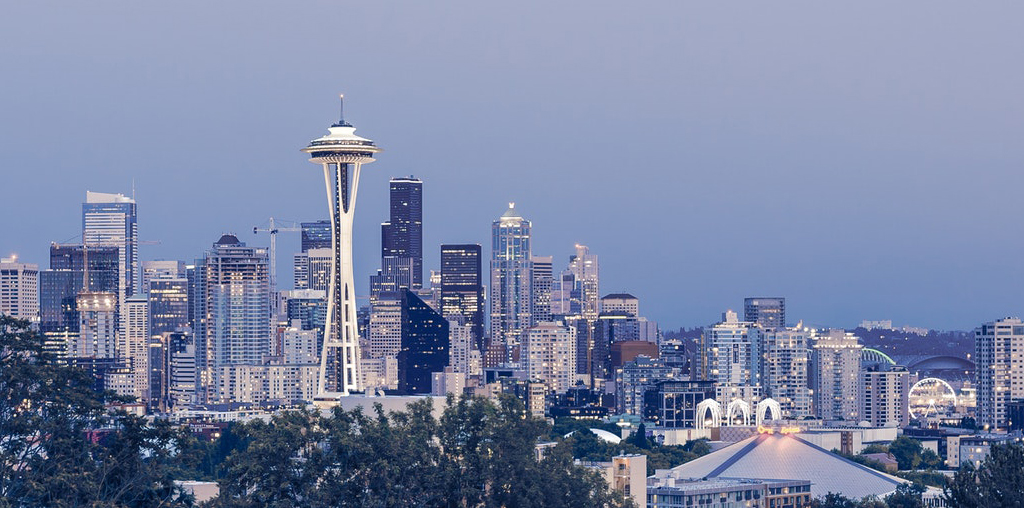
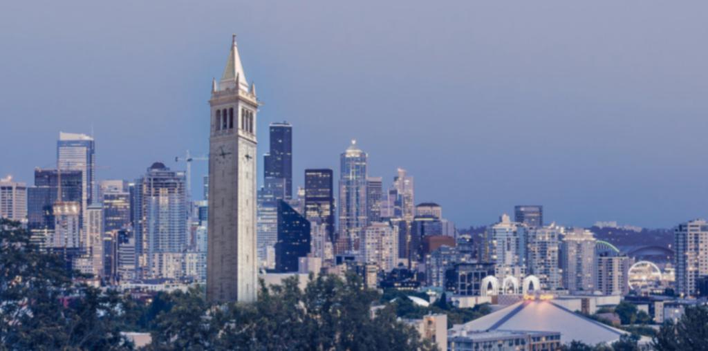
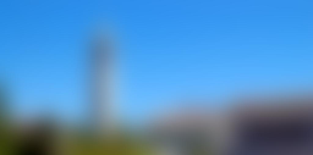
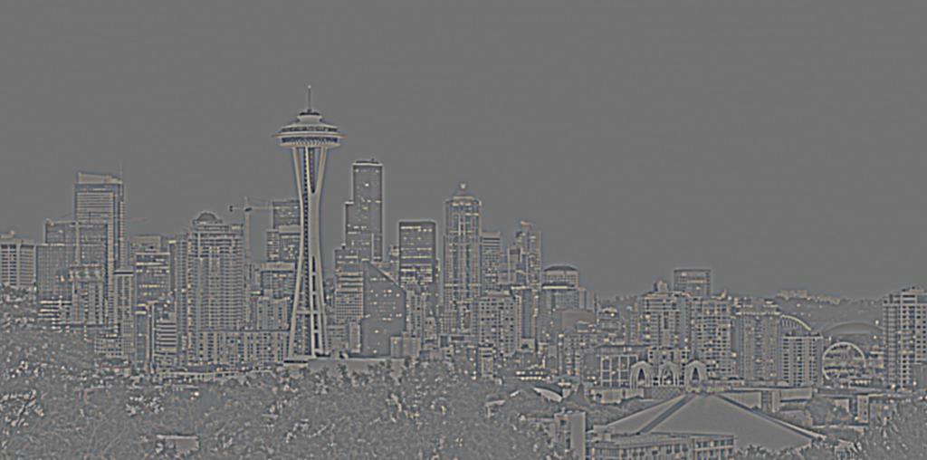
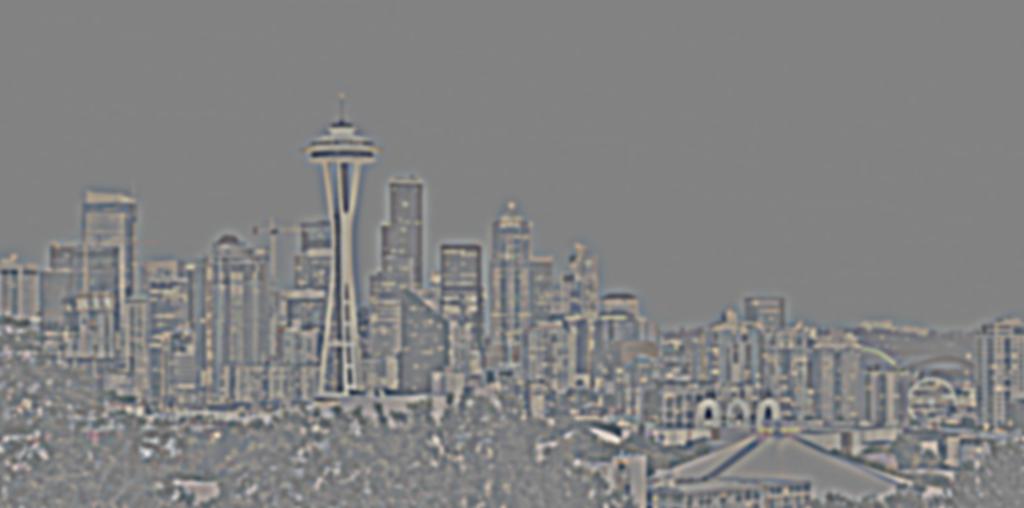
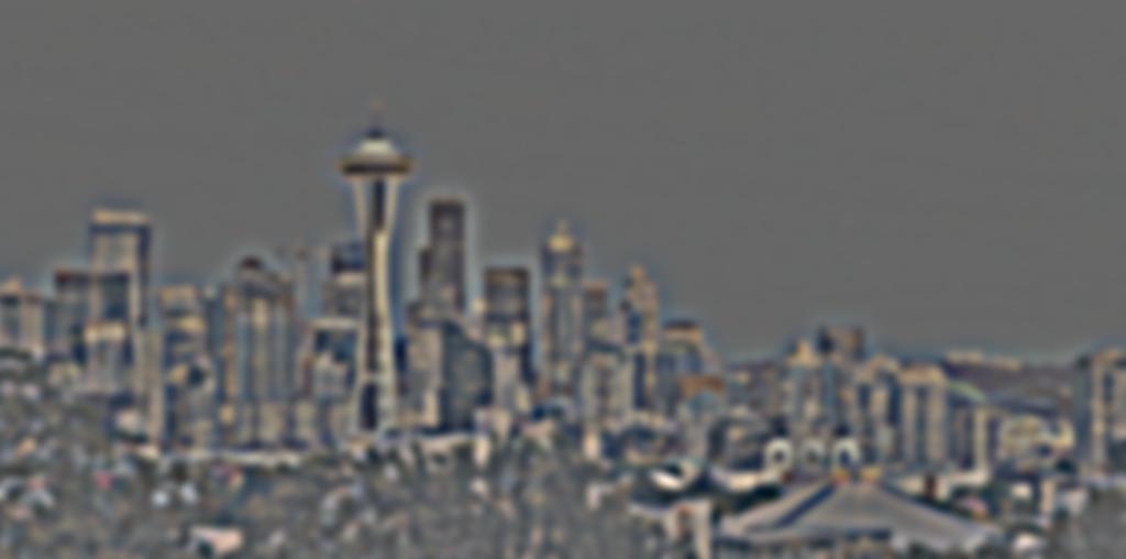
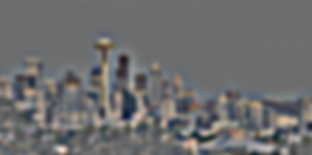
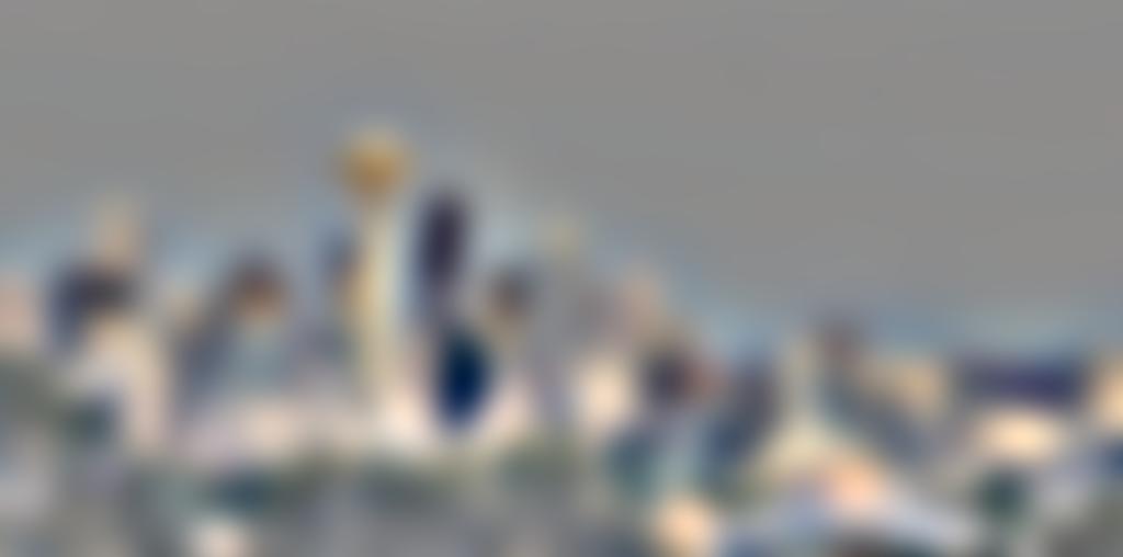
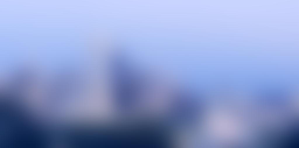
We also try replacing the Space Needle with the Campanile in the Seattle skyline.

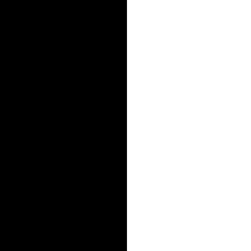
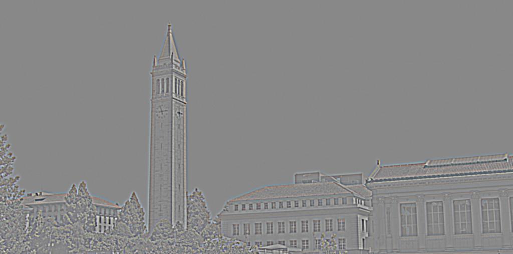
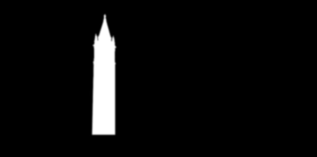
Below are the components used in the Poisson blend: the Laplacian stacks for the two images, as well as the Gaussian stack for the mask.

Part 2: Gradient Domain Fusion

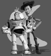
Part 2.1: Toy Problem

We will now explore the applications of gradient domain processing. Processing images in the gradient domain involves looking at the differences between neighboring pixels rather than directly on individual pixels. We first start with a toy example in which we try to reconstruct an image by computing the x and y gradients from an image. This boils down to a least squares optimization problem, in which we are minimizing the following objectives:

For source image s and output image v,

1) Minimize (v(x+1, y) - v(x, y)) - (s(x+1, y) - s(x, y)))²

2) Minimize (v(x, y+1) - v(x, y) - (s(x, y+1) - s(x, y)))²

3) Minimize (v(1, 1) - s(1, 1))²

Shown below are the results of the image reconstruction method.

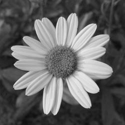
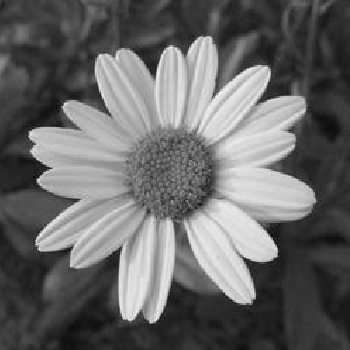
Part 2.2: Poisson Blending

We now implement Poisson blending, which will allow us to compose a seamlessly blended image from a source image and a target image in the gradient domain. The idea here is that, after cutting out one region of a source image and pasting it into a target image, we can match the gradients of the source and the target. In order to do this, we follow the method explained by Junyan in class:

We will be creating an output image v. For unmasked pixels, i.e. pixels in the target image t, we just set v_i equal to t_i. For masked pixels, however, we want to set the gradients of the mask equal to the gradients of the target image. We take the gradient to be the Laplacian filter, in this case:

0	-1	0
-1	4	-1
0	-1	0

If a pixel inside the mask has all four neighbors inside the mask, then we minimize the following constraint: ((v_i - v_j) - (s_i - s_j))². Otherwise, if any neighbor j is outside of the mask, we want to use the intensity value of the target image, i.e. we want to minimize ((v_i - t_j) - (s_i - s_j))².

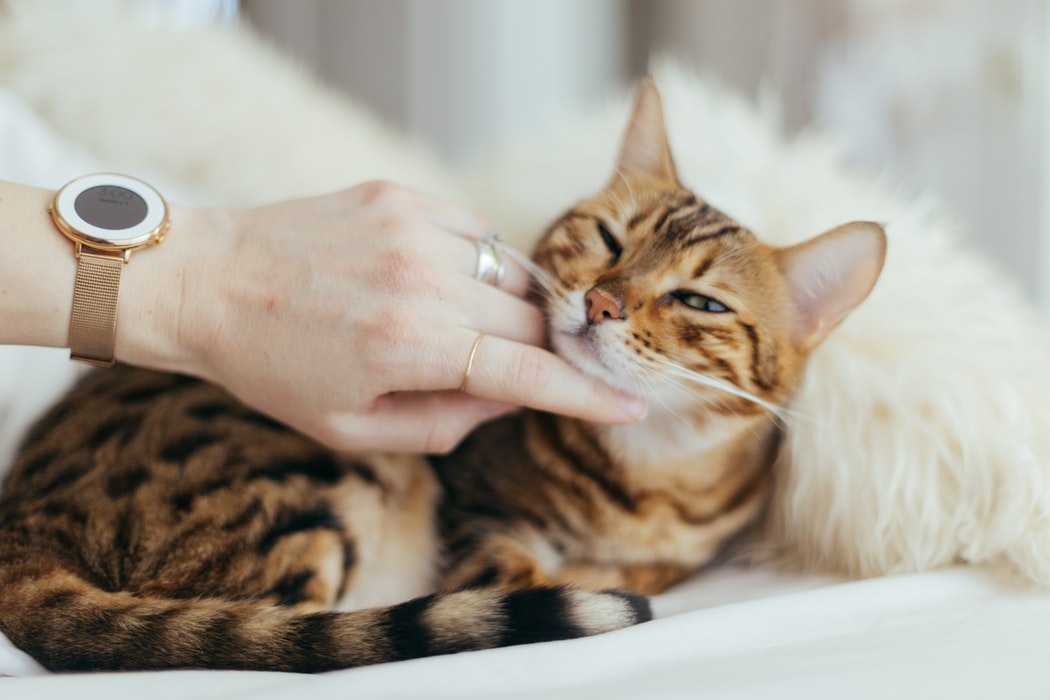
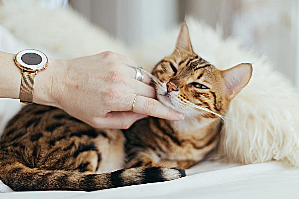
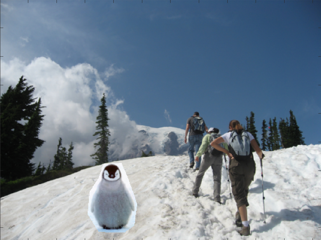
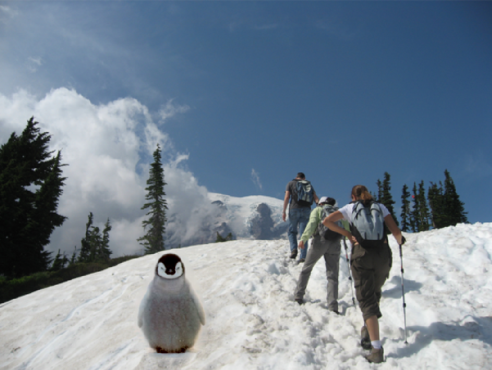
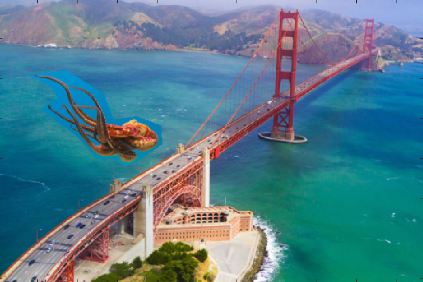
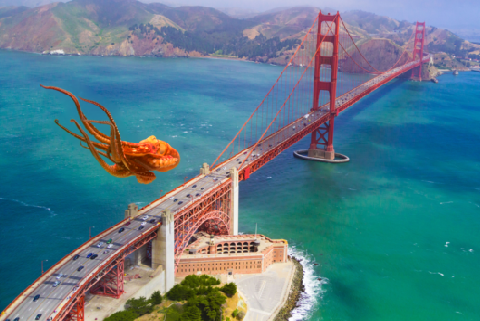
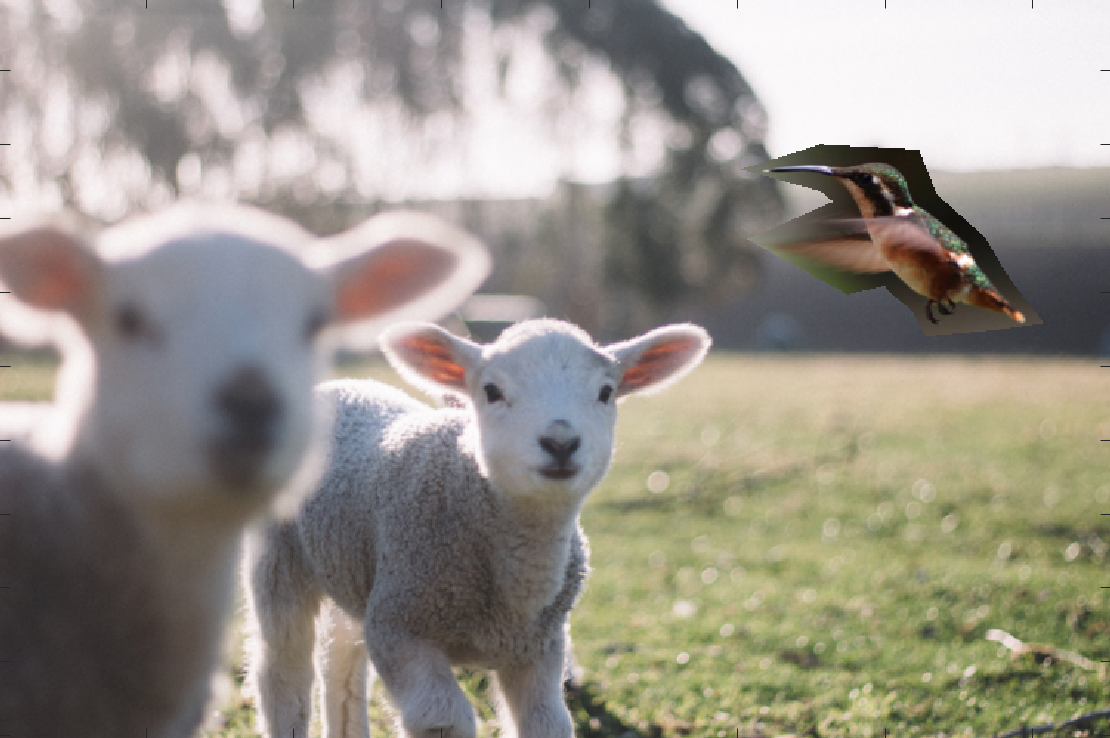
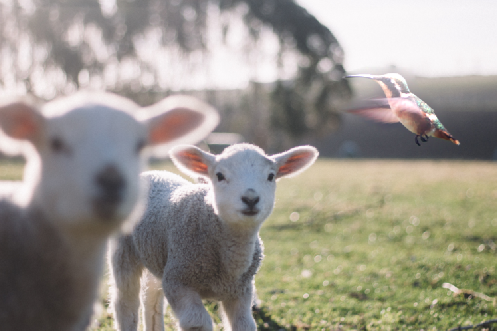
Shown below are the results of Poisson blends on different input images.

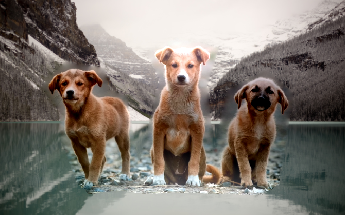
Finally, we try this Poisson blending technique with images we tried to blend with multiresolution blending, so we can compare the two.

A side-by-side comparison is shown below. We notice a pretty drastic color difference in the Poisson blended image. This color adjustment maintains the opaqueness of the dogs, while in the multiresolution blended image, the dogs are slightly transparent.