CS 194-26
Image Manipulation and Computational Photography
Project 3: Image Blending
Hemang Jangle, cs194-26-acv
Overview
In this project, we investigate different techniques for performing image blending. Part 1 of the project uses frequency domain analysis to sharpen blurry images, create hybrid images, and do seamless multiresolution blending. Part 2 of the project makes use of the gradient domain of images - a domain that represents images in terms of their horizontal and vertical derivatives. Because human visual perception places more importance on high frequencies of an image - ones that are captured well by gradients - we can perform almost flawless visual blending using the gradient domain.
Part 1
Sharpening Blurry Images
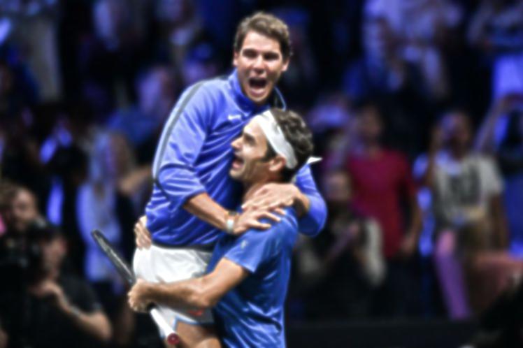
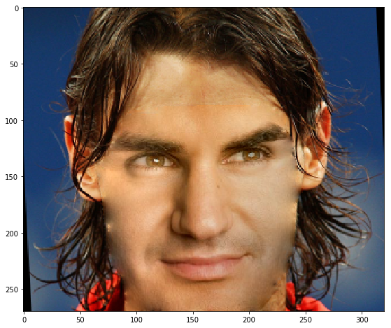
Here we use the 'unsharp filter' which uses the laplacian filter to find high frequency components of the image. Then, the high frequency components are added back to the image with a weight a - when a is larger than 0, we see a boost in the high frequencies. Here is a result from the infamous Fedal moment, a moment in time all tennis fans must see a little more clearly. A moment when The Swiss Maestro and The King of Clay came together to win the Laver Cup. In this example we set the sigma of the gaussian and a both at 2.
 Blurry
|
 Sharp
Sharp
|
Hybrid Images
Here we create hybrid images that appear as two different images, depending on the distance from which one observes them. The underlying concept behind this technique is that high frequencies dominate visual perception. When we take the high frequencies of one image and the low frequencies of a another, and composite them, we multiplex the dominant frequencies. At large distances, very high frequencies cannot be seen. While at low distances, low frequencies are not dominant.
We also need to specifically choose the cutoff frequencies of the filters that we apply to each separate image. Each pair of images has a different optimal setting because of change in visual features as well as image resolution. Here we report the sigma of the Gaussian used to to compute the low-pass filter for each image. This is inversely proportional to the cutoff frequency of the filter, because as sigma increases, we average over a larger region and lose more high frequencies. For the images below: in pairs of sigma_low and sigma_high: (50, 40), (45, 25), (3, 8).
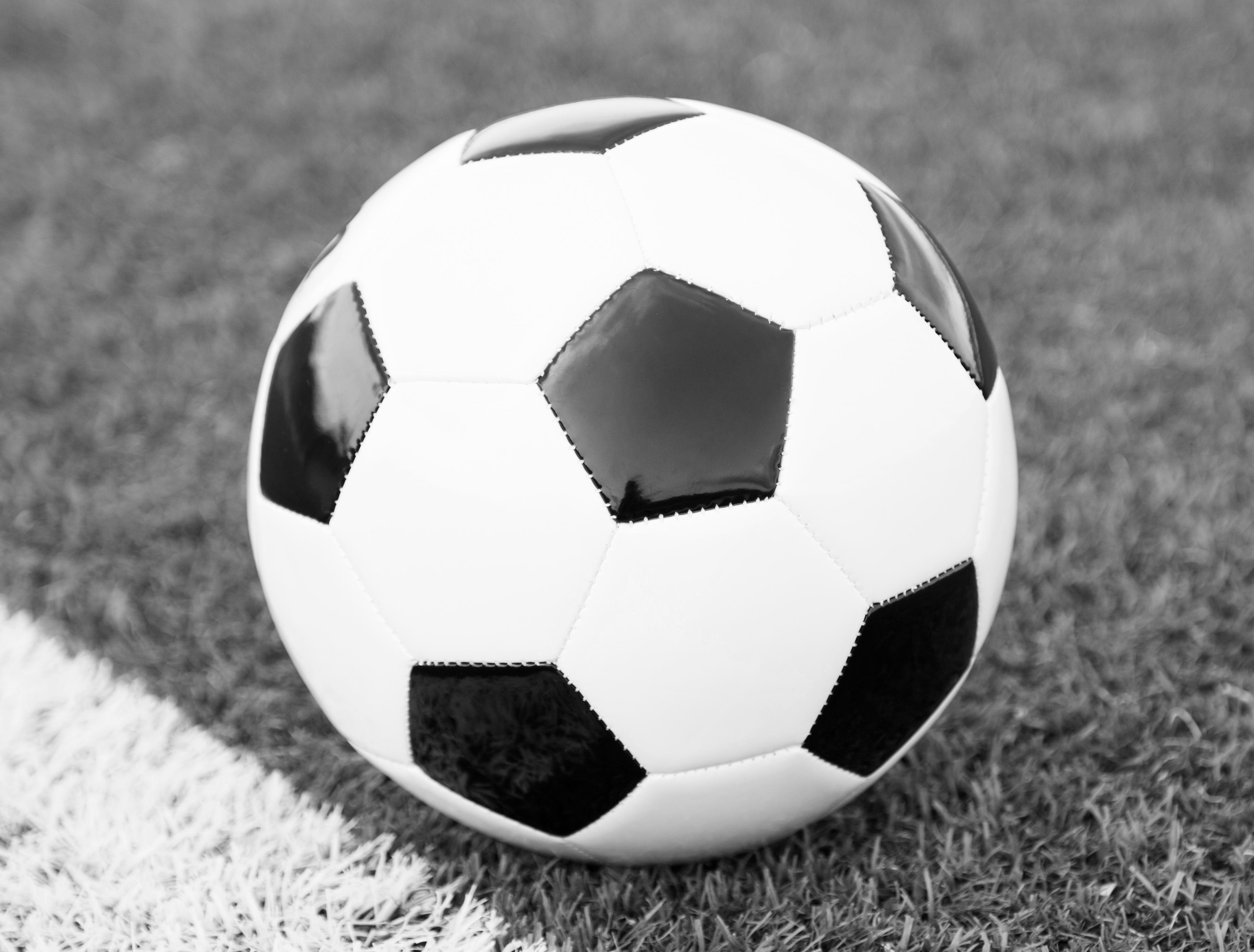 Original Soccer Ball
|
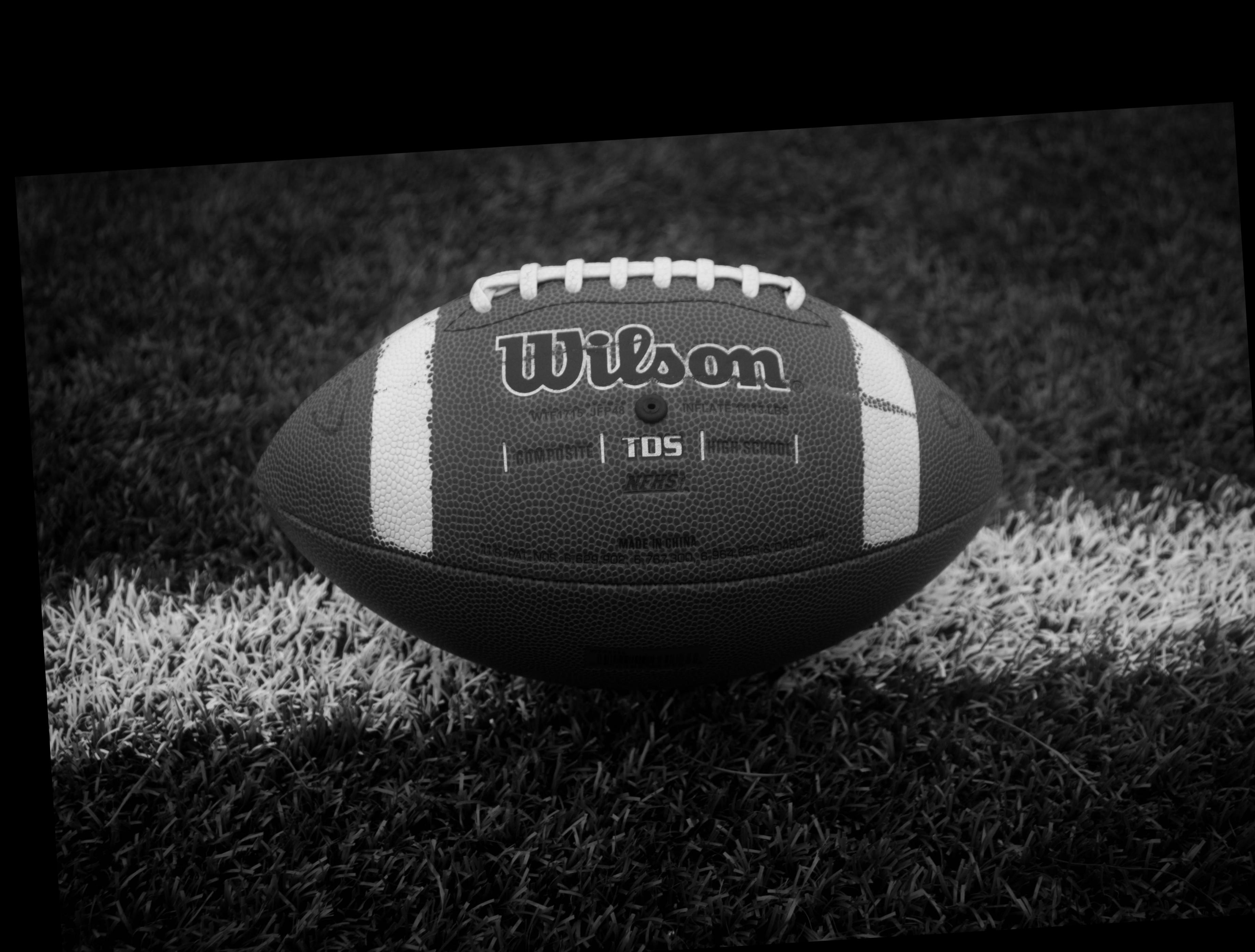 Original Football
|
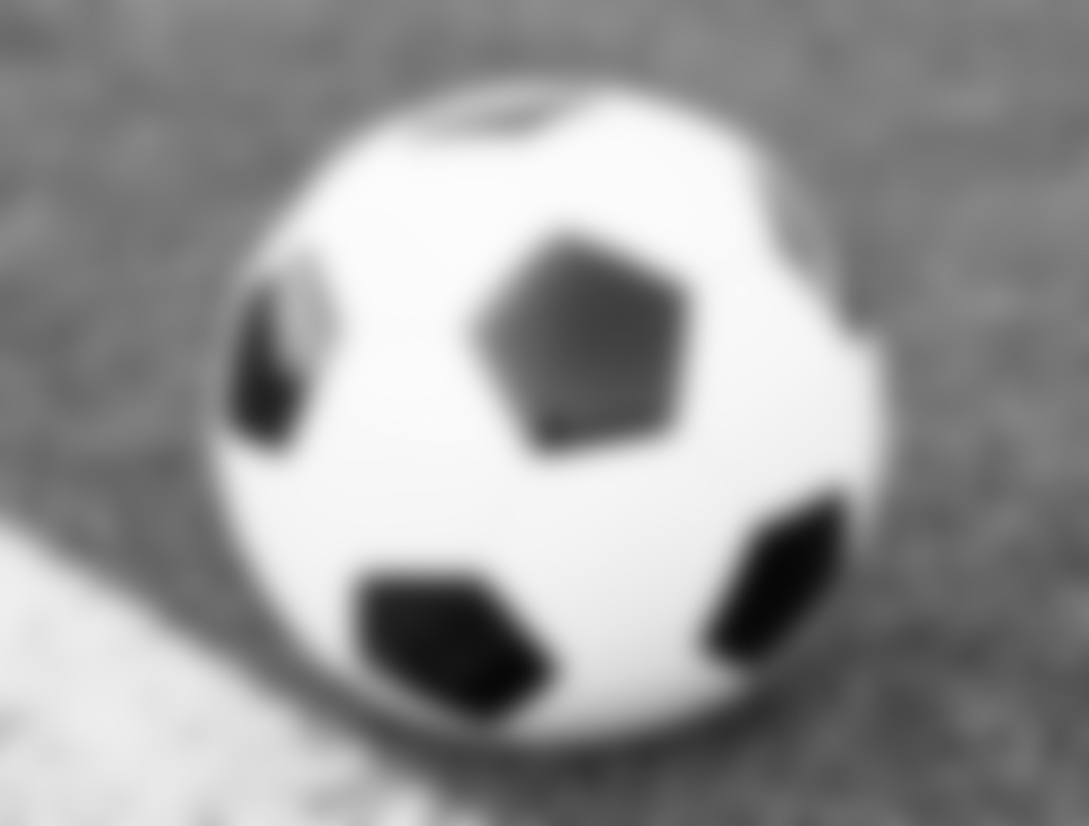 Low Frequencies of the Soccer Ball
|
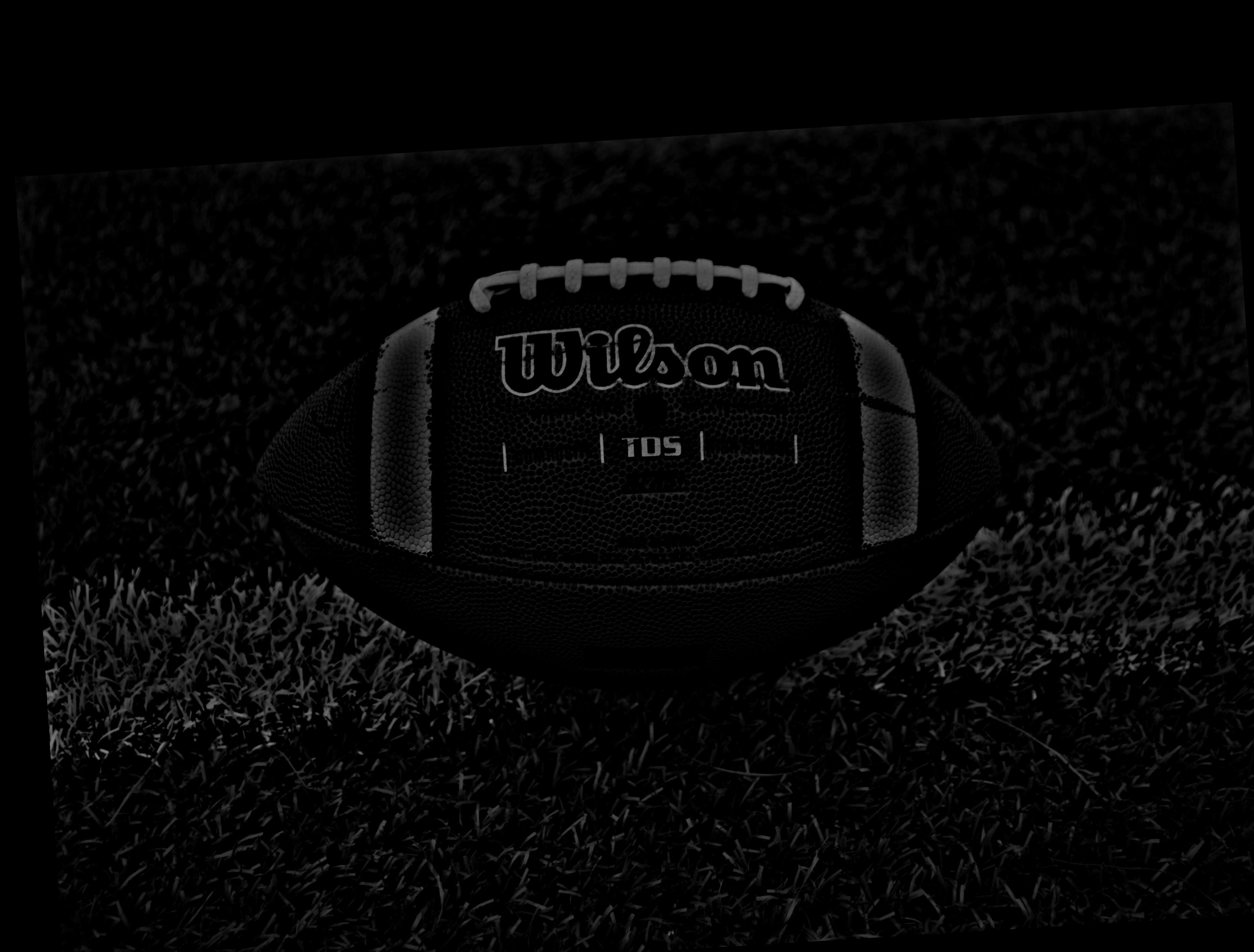 High Frequencies of the Football
|
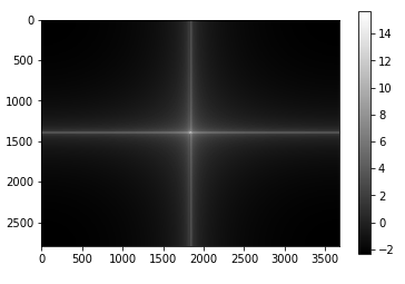 Fourier Transform of the Soccer Ball
|
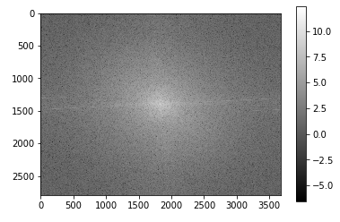 Fourier Transform of the Football
|
 Futball or Football?
|
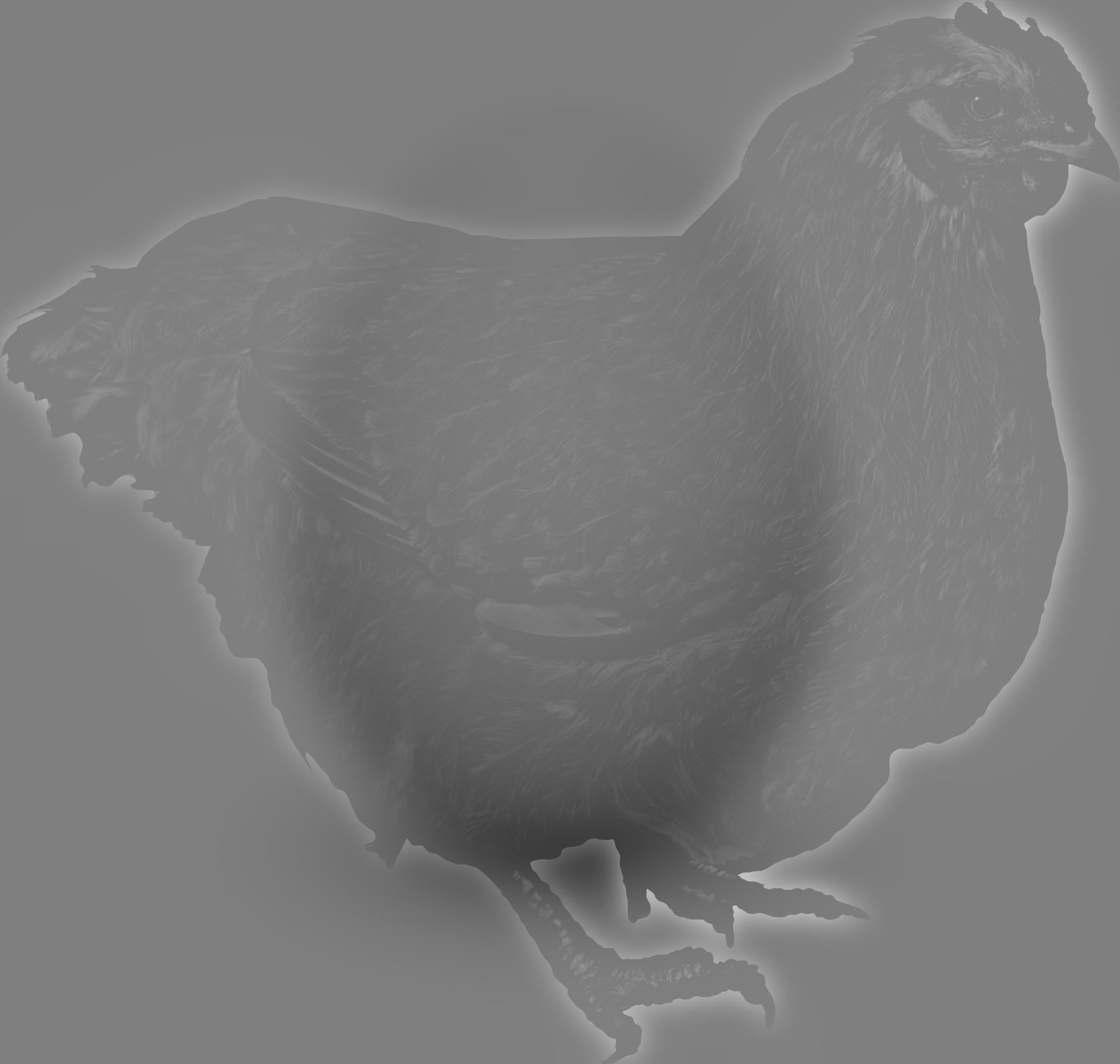 Which came first?
|
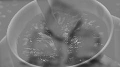 Like your coffee hot or cold?
|
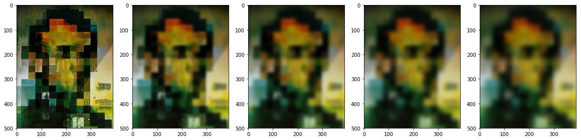
Gaussian and Laplacian Stacks
We can also make stacks of images that display different frequency content of an image. In a gaussian stack, we convolve with a gaussian at each level, so each successive image has a smaller active frequency range, in the low frequencies. In the laplacian stack, we take the difference of the images in the gaussian stack, and store them. Therefore, the images are band-pass filtered versions of the original. In a laplacian stack,we also store the most low-pass image to retain all the information in the original image. We first examine gaussian stacks of the Mona Lisa and Dali's painting of Lincoln and Gala to see different frequency level content. We display the laplacian stack in grayscale because it is easier to see the different bands.
 Lincoln Gaussian Stack
|
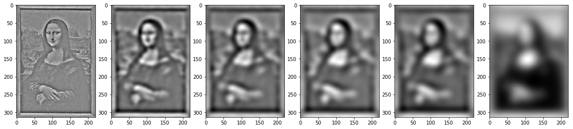 Mona Lisa Laplacian Stack
|
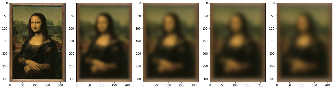 Mona Lisa Gaussian Stack
|
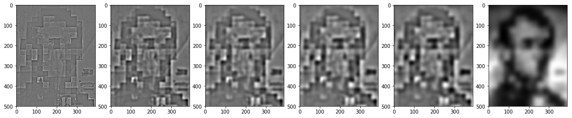 Lincoln Laplacian Stack
|
Here we examine the gaussian stack of the low-pass filtered soccer ball from the hybrid image above, and the laplacian stack of the high-pass filtered football from above. We can see the different frequency content.
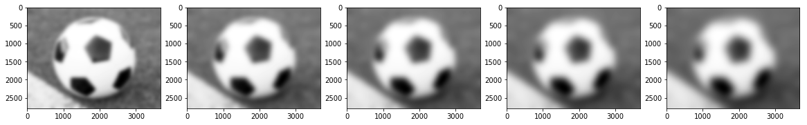 Soccer Ball Gaussian Stack
|
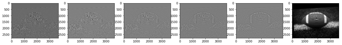 Football Laplacian Stack
|
MultiResolution Blending
We can use these stacks to also perform more seamless blending by blending together images at different frequency bands, and then compositing the result. Here are some examples!
 Original Federer
|
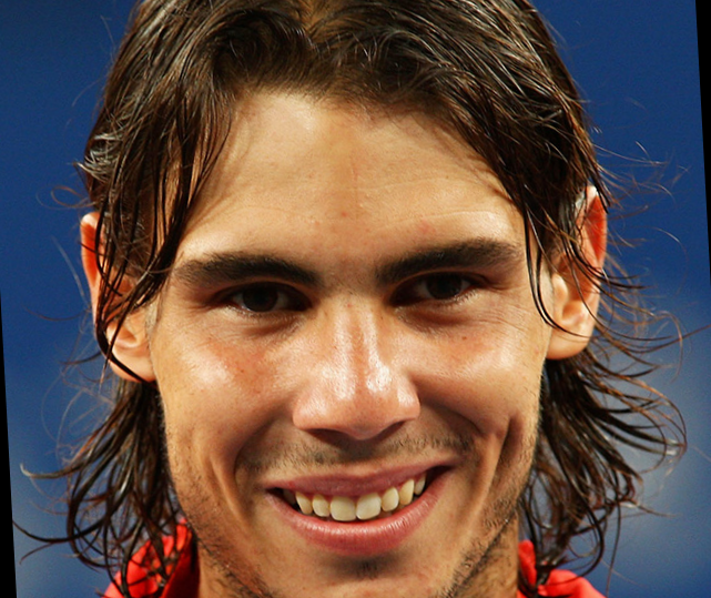 Original Nadal
|
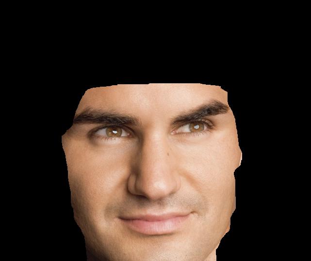 Federer Masked
|
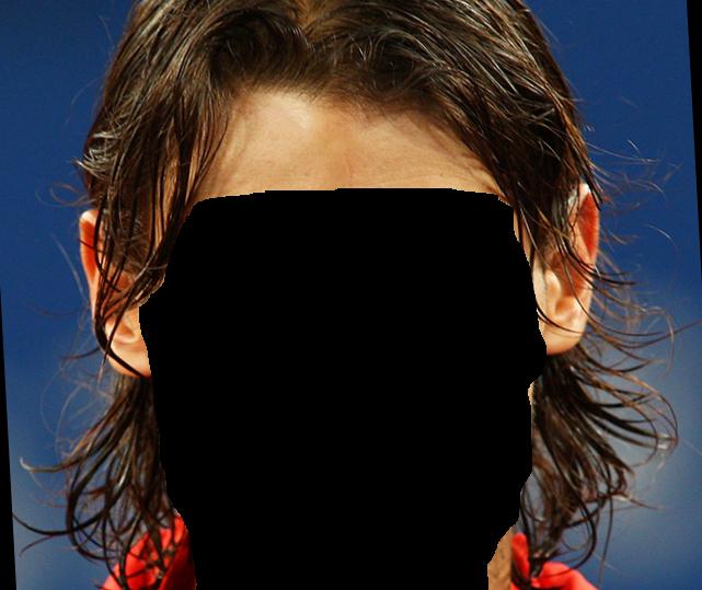 Nadal Masked
|
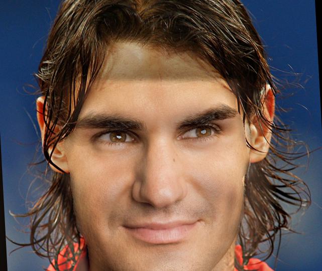 The Swiss King of Clay!
|
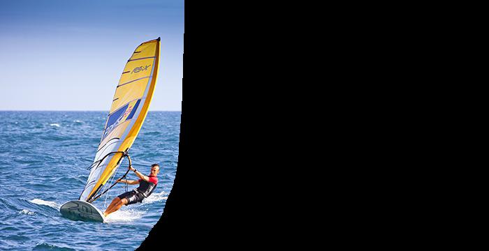 Windsurfer 1 Masked
|
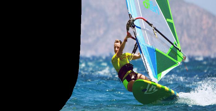 Windsurfer 2 Masked
|
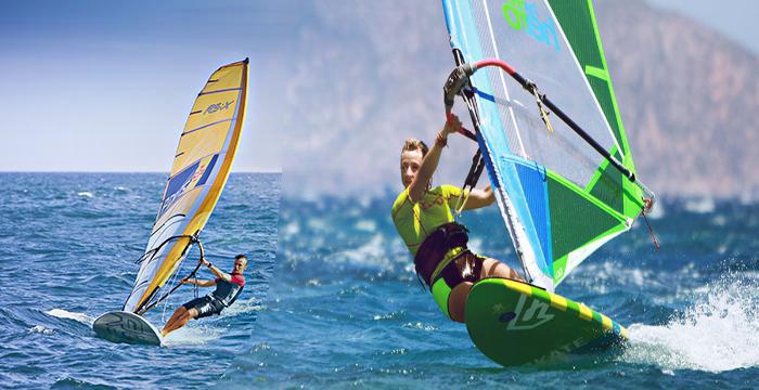 Windsurfers
|
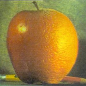 Oraple
|
Part 2: Gradient Domain Fusion
Gradient Domain Fusion is a technique for blending images that allows image transplantation by transferring the gradient representations of a source image to a target. Because we cannot perfect transfer the gradients of an image into a patch of another image because the surfaces of the mask boundary are almost always different, we can approximate a transplantation by minimizing the different in gradients in the source and target images. This gives us some very startling results.
In this first section we perform this optimization on a single image. Performing this correctly means we get the same image back, a good sanity check.
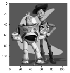 Input Image
|
 Reconstructed Image
|
A Treasure of Time and Money
Here we see the blending of a clock from the infamous Dali: The Persistence of Memory, and a treasure chest. Truly, this is the most valuable treasure in the world. We have to provide a slightly more precise mask to get the clock only. In general, the source and target regions should have a similar background region so that there are no sharp discontinuities in the output.
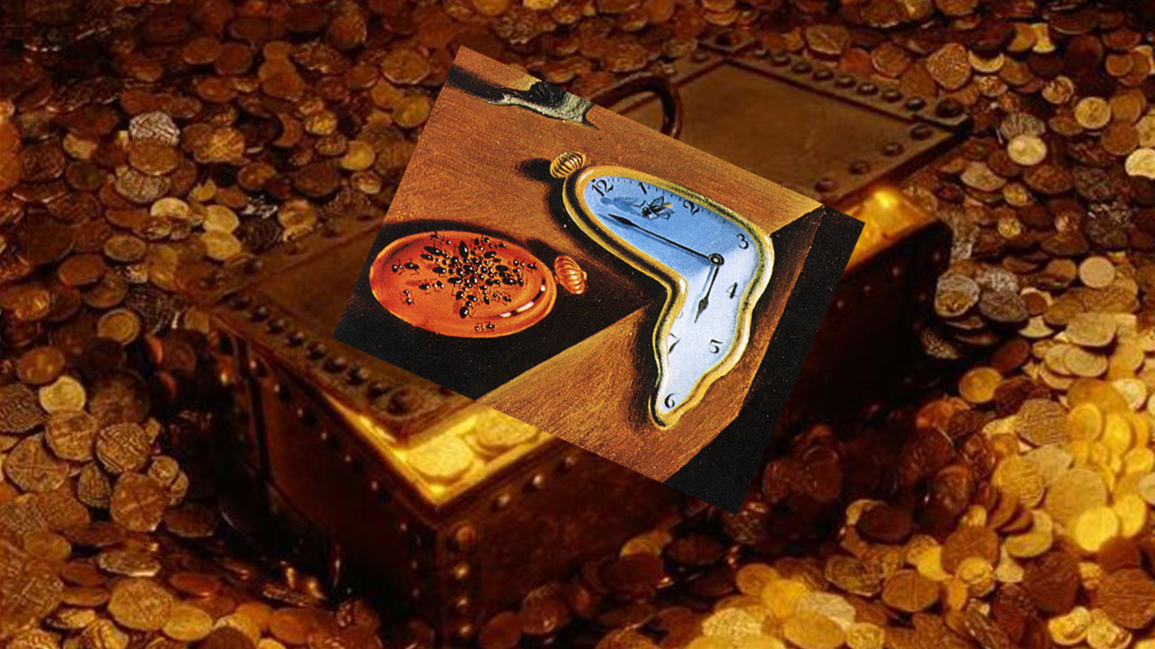 Source
|
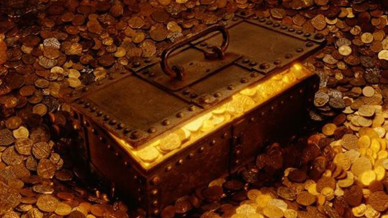 Target
|
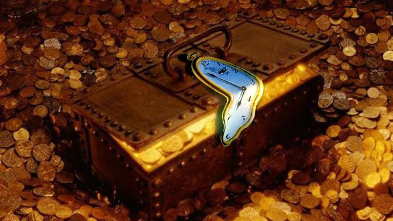 Output
|
Killer Whales in the Bay
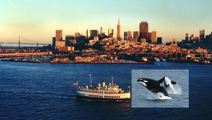 Source
|
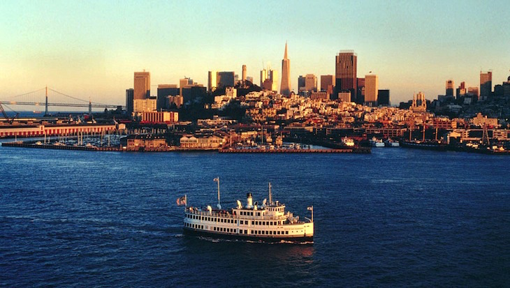 Target
|
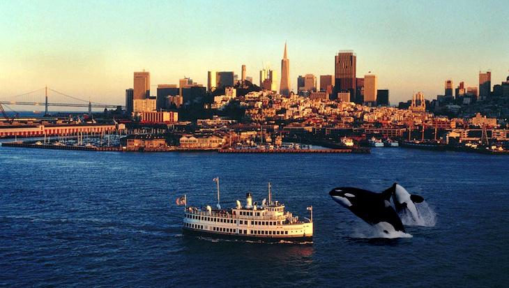 Output
|
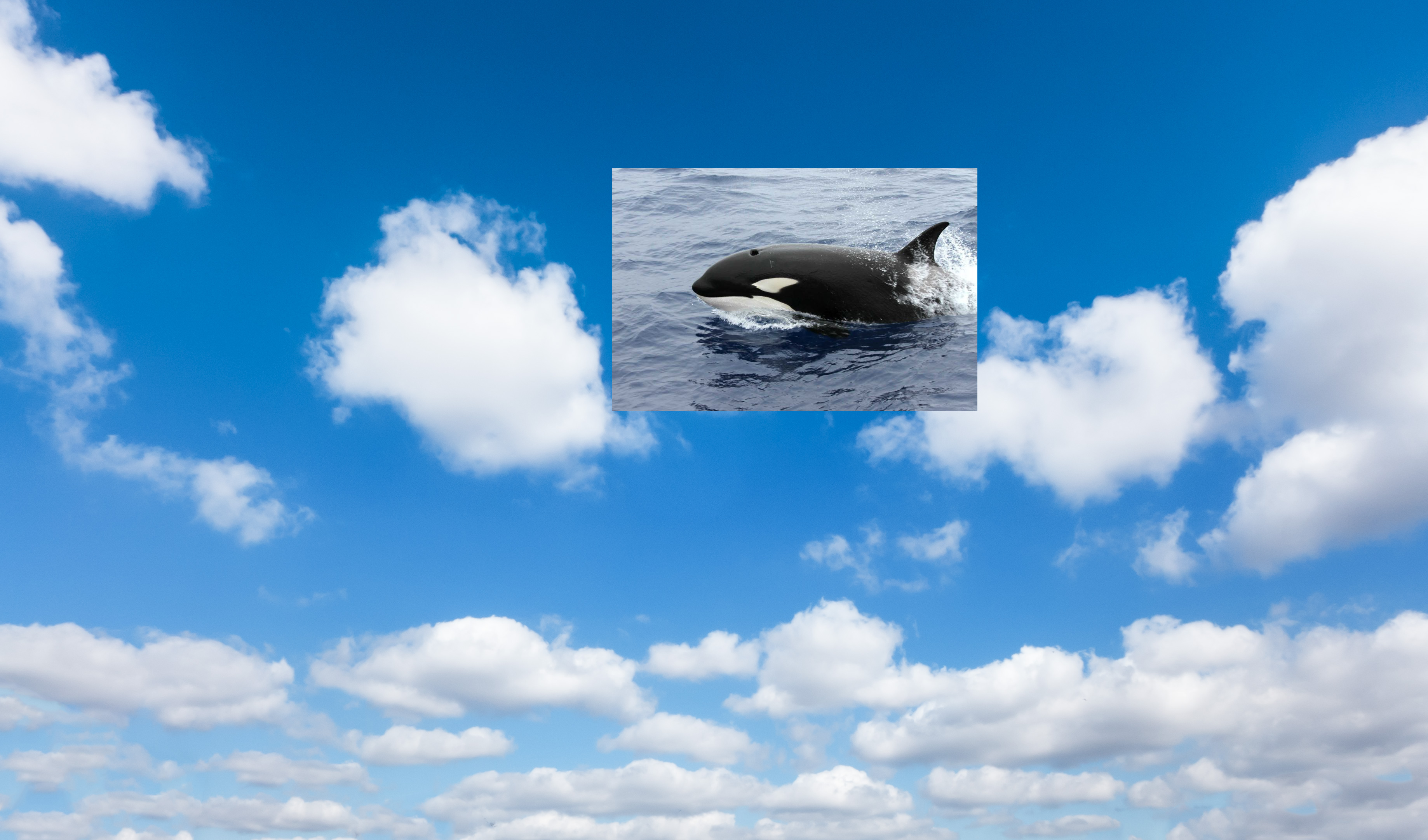
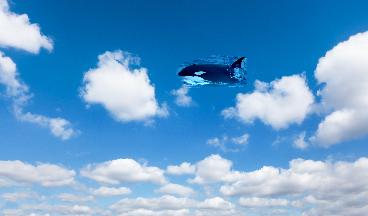
Killer Whale in the Sky
This is a failure case where we see discontinuities. This occurs because the background sky is completely constant whereas the water is a bit noisy. We can't blend these easily together. The pixelation seen also comes from resizing the whale too small.
 Source
|
 Target
|
 Output
|
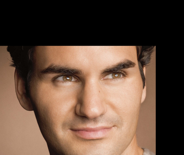
Federer Nadal Comparison
Here we compare the Federer Nadal blend from earlier to the blend using gradient domain fusion. The blend using gradient domain fusion works a lot better here because the borders between the foreheads is a lot smoother - because we have to satisfy the boundary constraint. Moreover, this blend can be categorized more cleanly as a patch insertion, where as something much smoother like the apple orange blend that benefits from alpha matting.
|
Federer
|
Nadal
|
|
MultiResolution Blend
|
 Gradient Domain Fusion
|