Project 3: Fun with frequencies (and gradients)
Introduction
While viewing an image as pixel values is the most straightforward way, understanding the image in the frequency domain can tell us a lot about the image and allow us to make many fun applications. In this two-part project, we will first play around with the frequency domain. While frequency domain is important, human vision is most sensitive towards edges, which can be captured by the image gradients. Therefore, in the second part of the project, we use a technique called Gradient Domain Blending to achieve some really fun applications.
Part One: Frequency Domain
1.1: Image Sharpening
Gaussian filter is arguably the most important filter in image processing. It removes the high frequency details in an image. However, if we subtract the filtered image from the pre-filtered image, we actually acquired the high frequency parts that gets filtered out. If we add this part back to the pre-filtered image, we achieve a very crude way of doing image sharpening.Below is a demonstration

A dog before sharpening
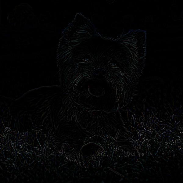
The part lost via filtering
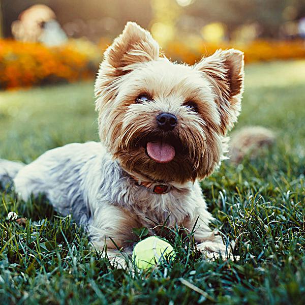
After sharpening
Here we have the sigma value in the Gaussian filter to be 2, if we choose a larger sigma, we would have more high frequency details under enhancement but 2 is the most aesthetically pleasing value for this particular image. Here is a look at the sharpened details
1.2: Hybrid images
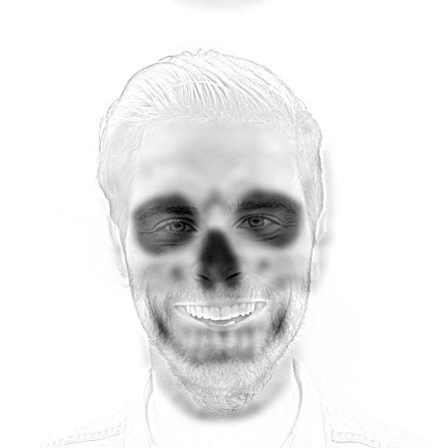
In the previous application, we are enhence the high frequency part of an image and add back to the original image. If we take out the high frequency image and add it to a different image (or the lower frequency part of it) we can have some very interesting hybrid images. For example, if we have the following two images
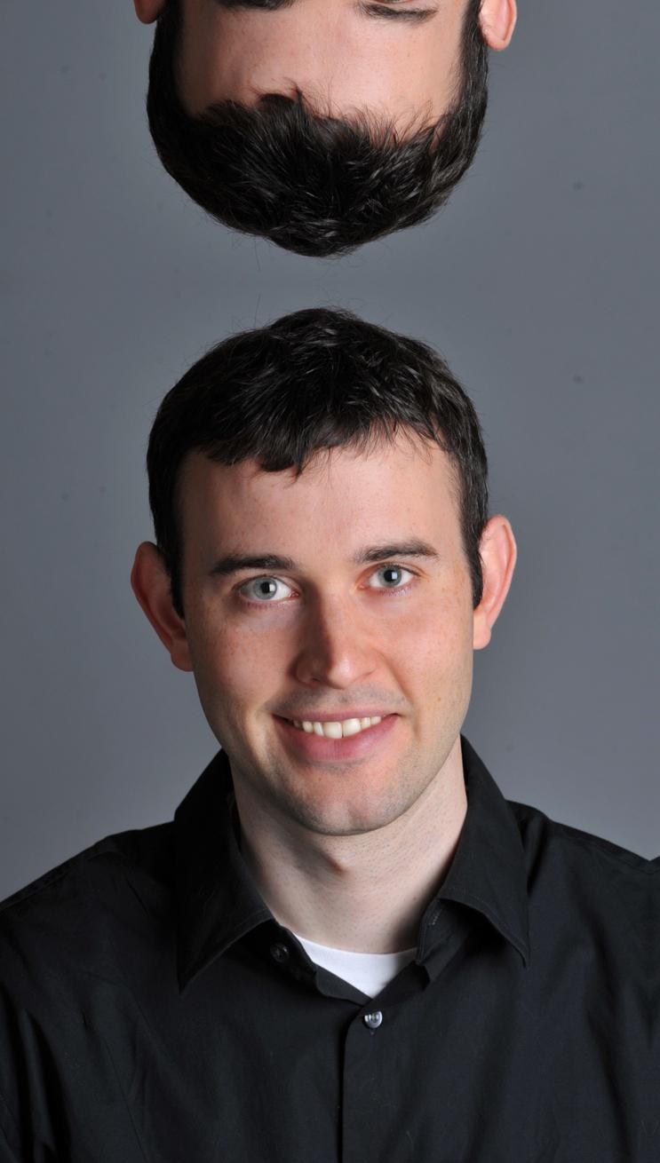
Derek
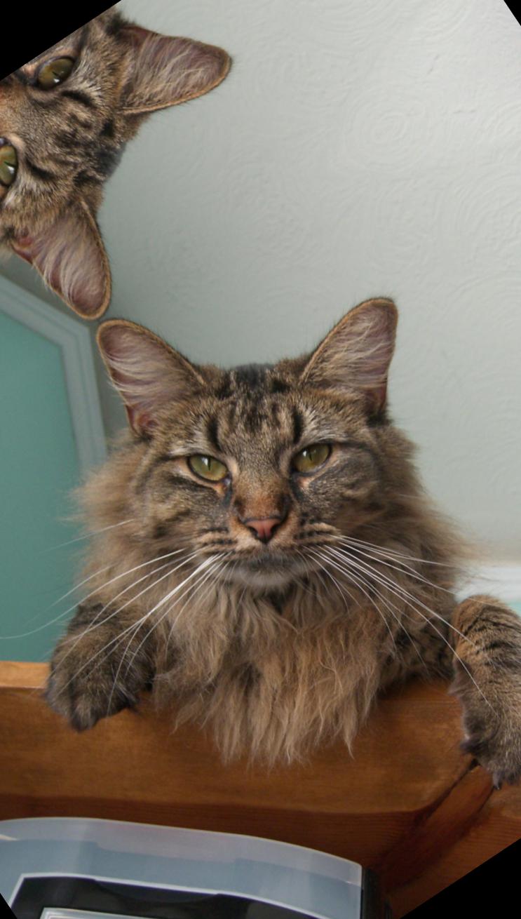
Nutmeg
We notice that Kobe has a more homogeneous look but the mamba has more high frequency parts (its scaly pattern). We can apply a low-pass filter on Kobe and a high-pass filter on mamba. After tuning the threshold for the two filters, we have the following result.
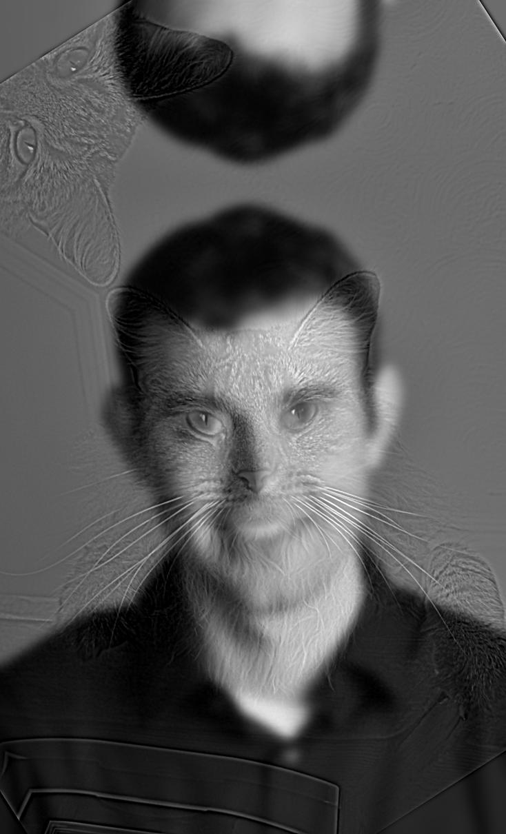
Gray version
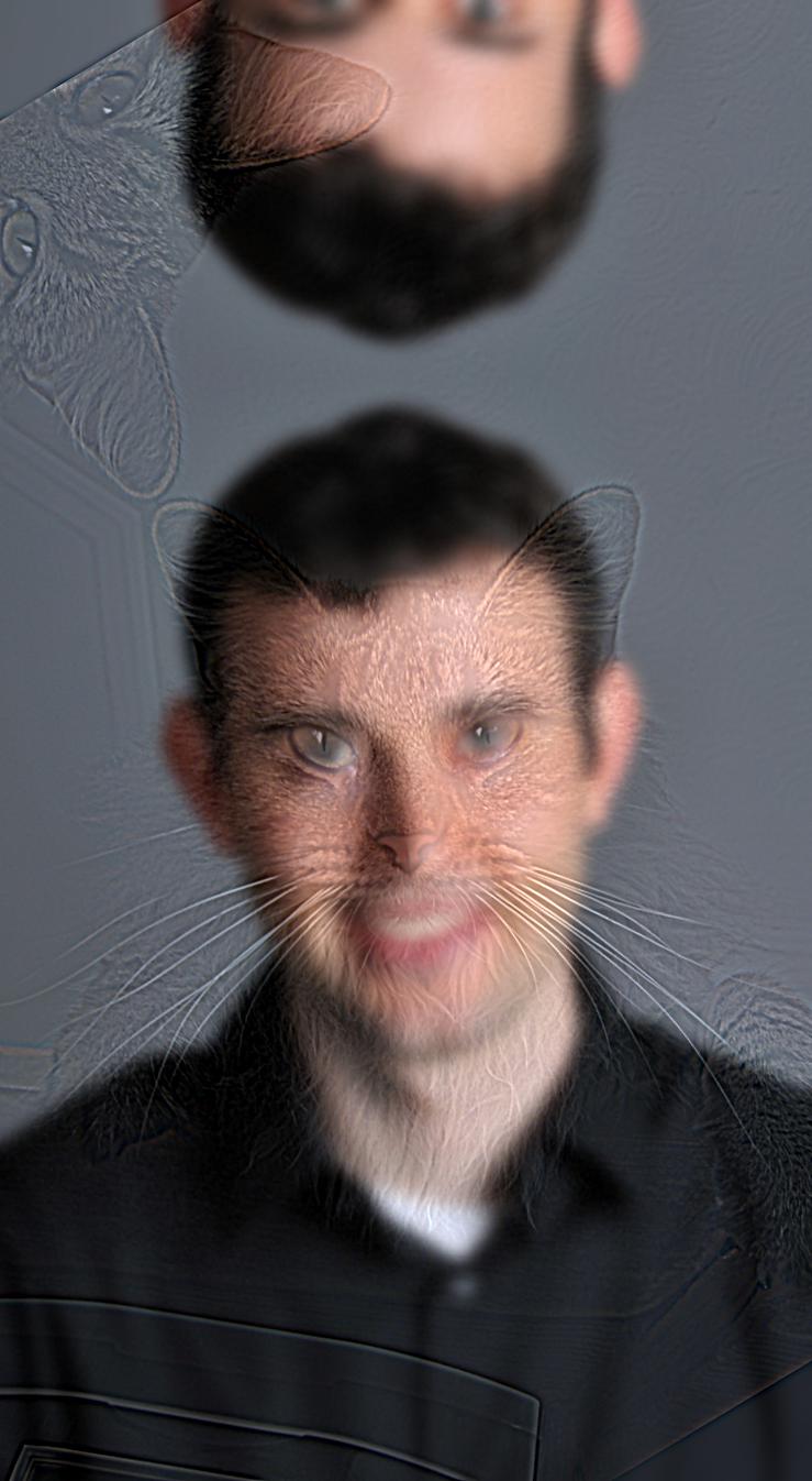
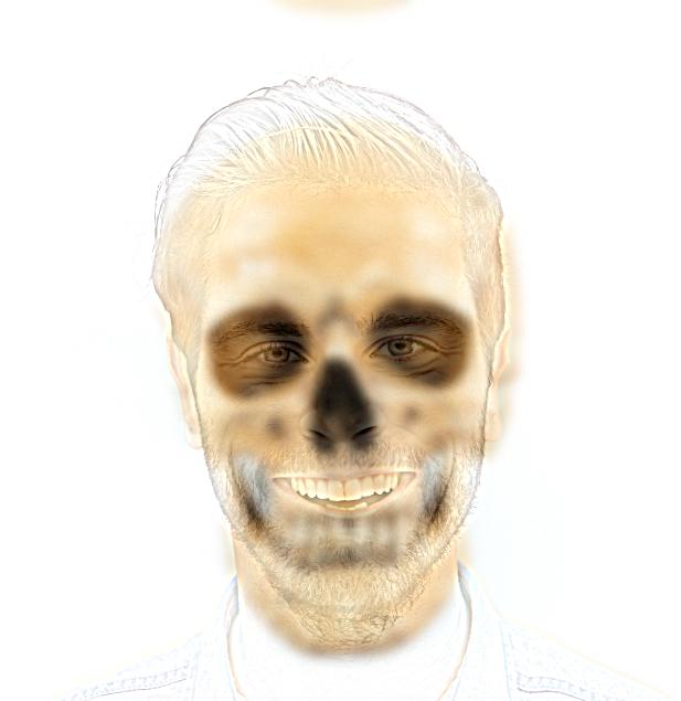
Color version
Personally I like the gray version better since the if colored, the low frequency image becomes more predominant perception-wise, the effect is not as astonishing. We can use fourier transform to examine what is actually going on
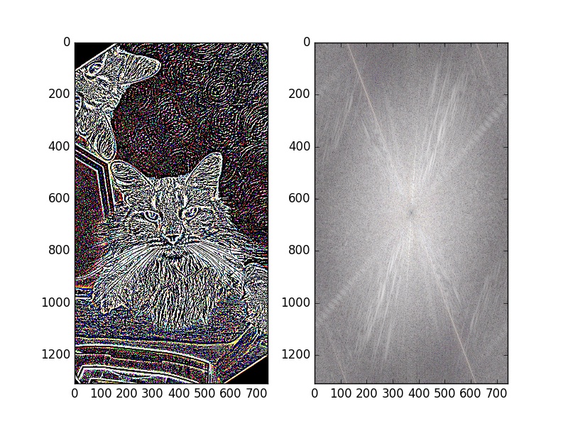
High pass filtered image and its 2D fourier transform plot. We can see the center of the plot is relatively dark since the low frequency part is filtered out. Also the plot has brightness in the entire image since there are prominent lines in many directions in the original image.
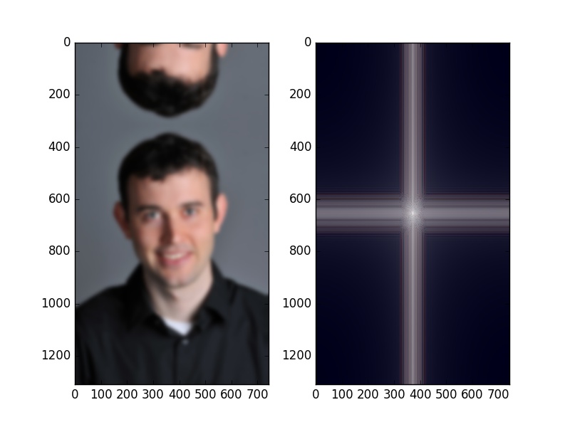
Low pass filtered image and its 2D fourier transfrom plot. The center of the plot is brighter in this case
Here are two more examples:
Underneath Us (Gray version)
Underneath Us (Color version)
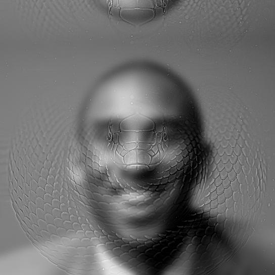
Mamba Spirit (Gray version)
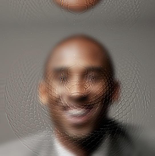
Mamba Spirit (Color version)
Unfortunately Kobe and mamba example did not turn out so well, because the hybrid technique is rather crude and does not factor into account that different faces have different geometry. An direct overlay produces ugly artifacts. An improvement would be warp the mamba first before hybrid them.
1.3: Gaussian and Laplacian stack
In the previous example, we analyzed the high-pass and low-pass filtered image. However, if instead of two levels, we do it in multiple levels, we end up with a stack of images, each corresponding to a different frequency range. For example, if we use gaussian filter on one image 6 times, each time use a sigma value twice the level index, we have
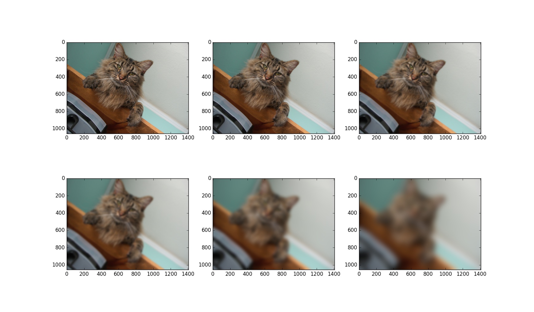
6-level Gaussian stack
If we take the previous gaussian stack and find the difference between each level, we obtain a Laplacian stack, as the following
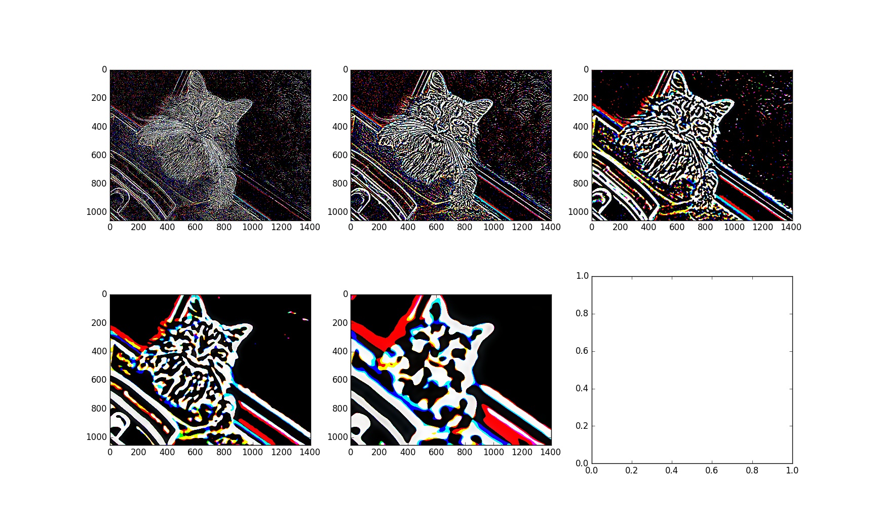
5-level Laplacian stack
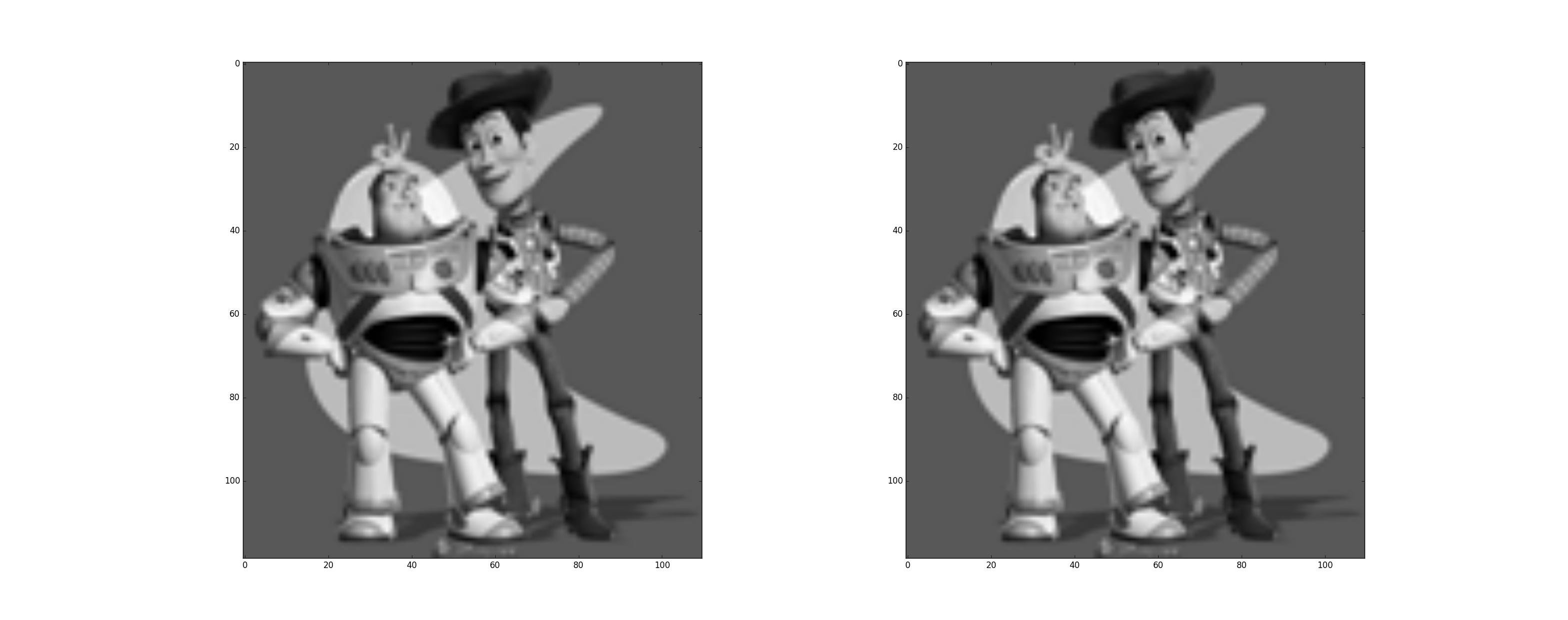
Laplacian gives us a really good idea of image component in each frequency range. And we can use the plot of Laplacian stack to analyze our hybrid image. For example,
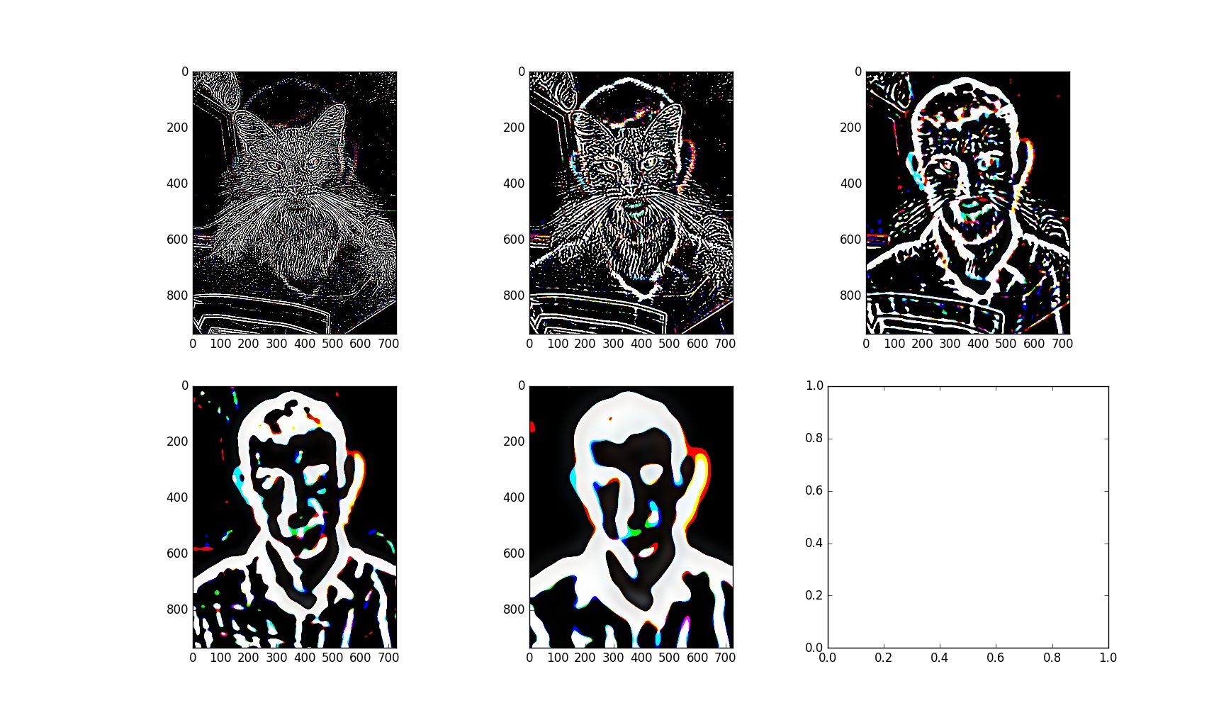
We can observe that at higher frequency, cat image predominates the person. At lower frequency, person dominates over the cat.
1.4: Multi-resolution Blending
One application with Gaussian stack is smooth blending. In the scenario if we want to cut and paste one image onto another, direct substition of pixels will often results in a very abrupt and ugly seam. However, there are many different techniques that allows us to achieve natural and smoothing blending over the edge. Multi-resolution blending, or blending with Gaussian mask is one of them.
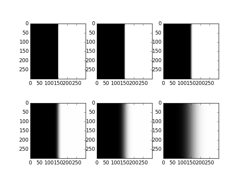
6-level Gaussian Mask
Instead of using one binary mask and two single images, we turn the images into Laplacian stacks, and use mask of corresponding Gaussian levels to blend images of corresponding Laplacian level. Finally, we combine the blended Gaussian component into one single image.
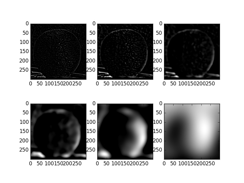
6-level Laplacian of orange. Apply the corresponding Gaussian mask on each level then add to the corresponding level of the other image.
Finally, we can achieve the following result:
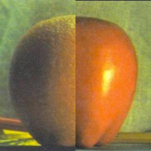
Direct pixel substitution
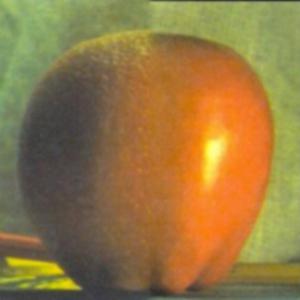
Gaussian Blend
Here are some other examples:
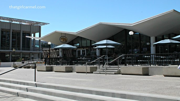
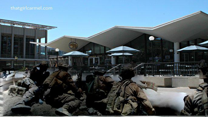
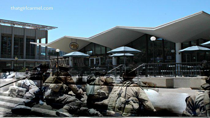
Golden Bear Cafe

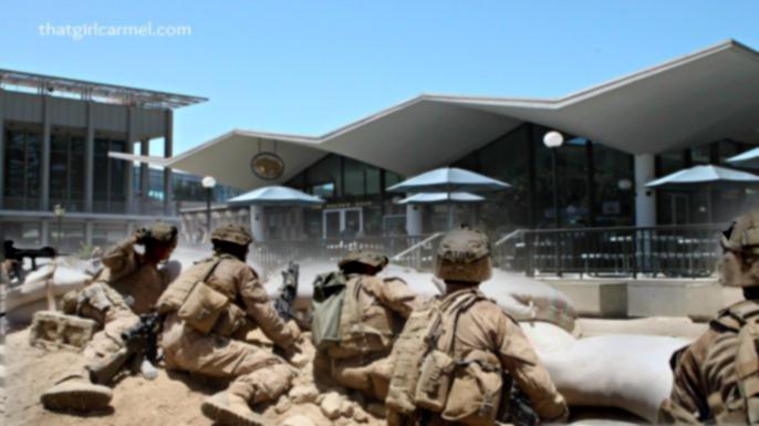
War
Berkeley in 2046
Arrival
Departure
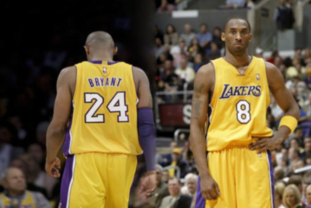
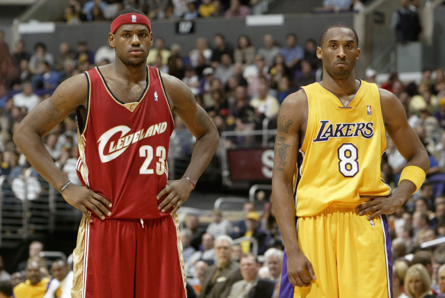
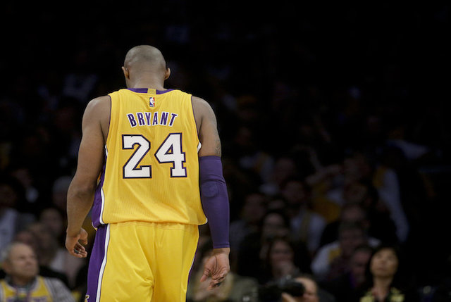
24 vs 8
Part Two: Gradient Domain Blending
Brief Outline
While frequency domain provides a very detailed understanding of an image in different frequency ranges, we usually pay more attention to higher frequencies since human vision is more perceptive of edges. To capture the edge information, image gradient is a good way to go. Therefore, gradient domain blending is a good alternative to frequency domain blending.
Specifically, we define a mask for the source image we want to blend onto the target image. Within the mask, we ensure that the image gradients match those of the source image at the same position. Outside of the mask, we simply copy over the pixel values in the target image at the same position. To ensure a smooth transition, we impose constraints that on the boundary of the mask, the result pixel values should equal to that of target image at the same position.
Toy Problem
Before we proceed about blending, we solve toy problem of image restoration. We are given a grayscale image s on the left. To restore an image f via gradients, we need to ensure that for every pixel f(x,y), the derivative on x-direction should match that of the original image, i.e. f'(x,y)=s'(x,y). In discrete sense, this means f(x+1,y) - f(x,y)=s(x+1,y)-s(x,y). Similarly, we match the y-derivative by imposing f(x,y+1) - f(x,y)=s(x,y+1)-s(x,y). To ensure the result image has the same intensity levels, we have one additional constraint: f(0,0) = s(0,0).
Implementation-wise, this amounts to solve a least square problem Ax = b where x is the pixel values in x, A stores appropriate coeffients to enforce the constrants, b stores the appropriate values for all s(x+1,y)-s(x,y) and s(x,y+1)-s(x,y). The result is the following:
original and restored image. L2-norm of difference = 0.000317018500698
Poisson Blend
Now to solve the actual blending question, we again solve a least square question Ax = b. x is again the pixel values within the mask that we need to solve for. A is the coefficient matrix to enforce the constraints. Specifically, we use a Laplacian kernel here so for pixel at (x,y), the corresponding A row would have to achieve (f(x,y)-f(x+1,y))+(f(x,y)-f(x-1,y))+(f(x,y)-f(x,y+1))+(f(x,y)-f(x,y-1)), assuming all four neighbours of (x,y) are within the mask. Otherwise, we simply have it to be zero. Then, b is the corresponding constraint values. Here is a demonstration of results.
To blend the penguin onto the background, we first create a mask for the source image
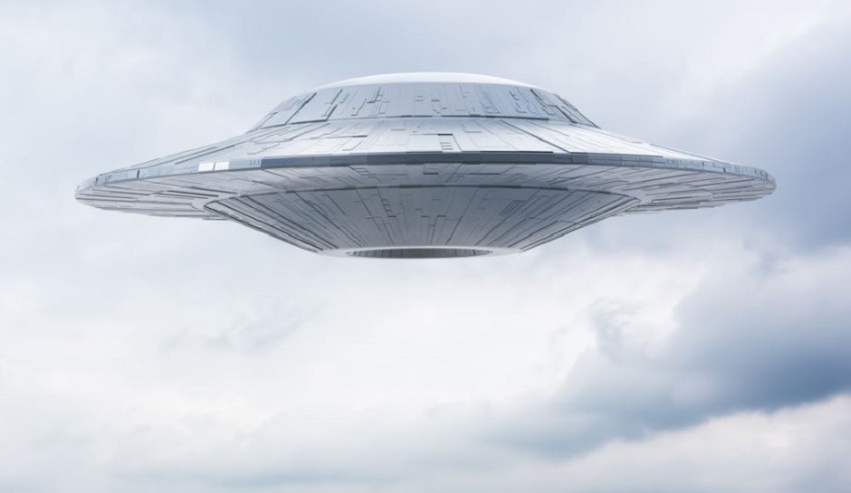
Source image
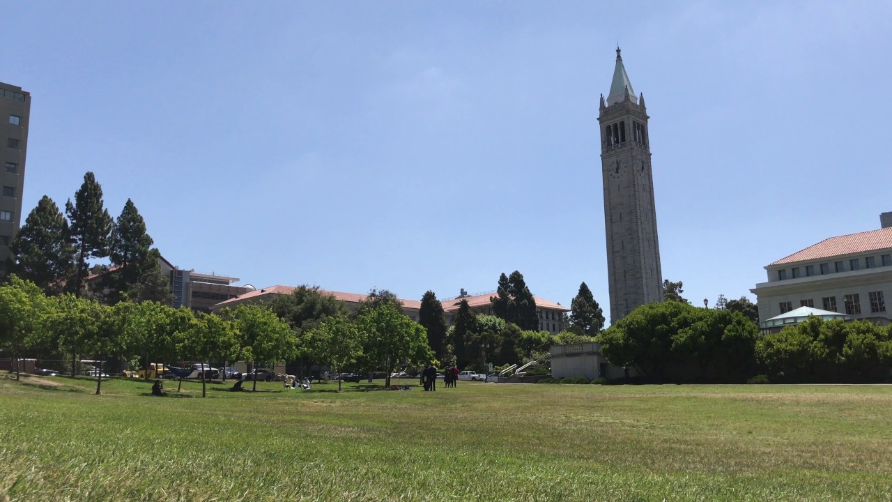
Target Background
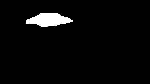
source mask
Then we solve the least square problem and we have:
Result of direct cut and paste
blending result
Here are two other examples
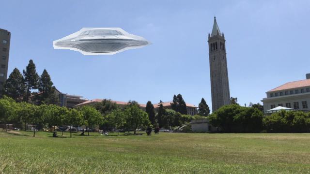
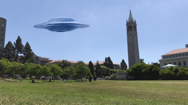
A normal day in Berkeley
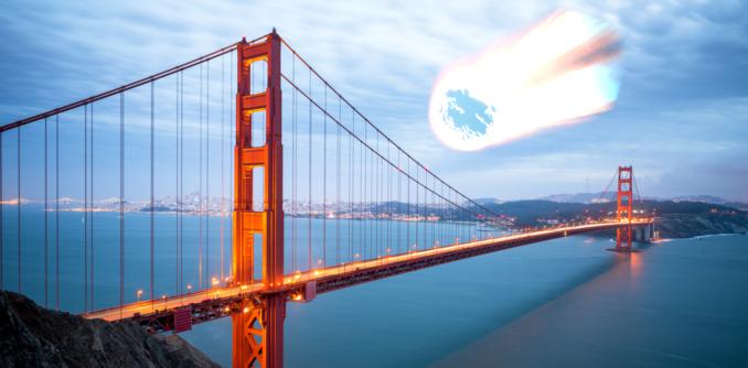
Cold Star
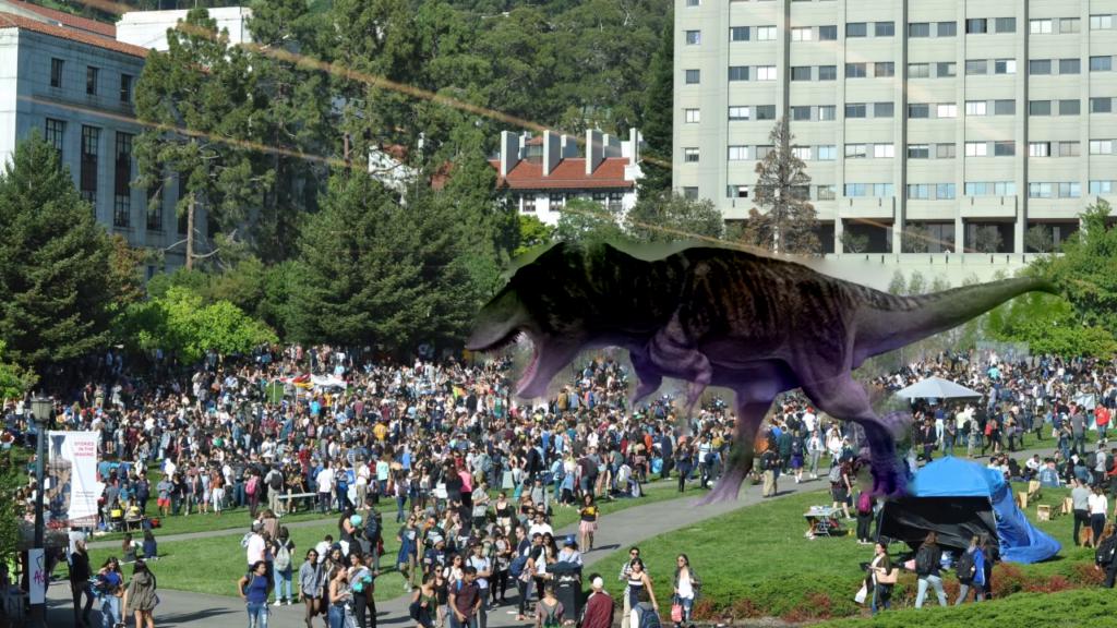
Notice that the effect of the first image is not so great since the color of the dinosaur looks off. This is because when we are trying to blend the dinosaur into the crowd, which has complex colors, our constraints are such that the edge will have the same color as the crowd. Hence, this constraint forces the color of the dinosaur to change. With gradient domain blending, the best effect is achieved when the background of the source image has similar color as the target image, as does the UFO and campanile.
Poisson Blend vs Laplacian Blend
Now we can compare and contrast the effect of poisson blending and Laplacian Blending
Laplacian Blending
Poisson Blending
We can observe that in Laplacian Blending, the color of both images are better preserved. However, for the exact same reason, the boundary between two images in Laplacian blending has a faded white artifact. This does not exist in poisson blending, but the cost is a worse color scheme for Poisson blending
Bells and Whistles: Mix Blending
While doing Poisson blending, we force the result to follow the gradients in the source image, however, if for a pixel at (x,y), we follow either the gradient in the source image or the target image, whichever is greater, we achieve something called Mixed Gradient Blending. This is sensible because we want to preserve the general features in both images. Here is a demonstration:
Poisson Blending
Mix Blending
In both cases, we observe the edge color bleeding effect as we saw in the dinosaur case. Here we however observe that the stairs are observable in Mix Blending. This is because the stairs are example of strong edge presence, hence in mix blending, their gradients are selected as constraint values.