CS194 Project 3 by Arnav Vaid

Part 1.1

Unsharp masking is a process where one convolves a gaussian filter across an image to obtain a low-passed version of the photo. Then, one can subtract a fraction of this low-passed version from the original photo, obtaining an image with sharper borders. An example is shown below:

Regular Image

Sharpened Image

Part 1.2

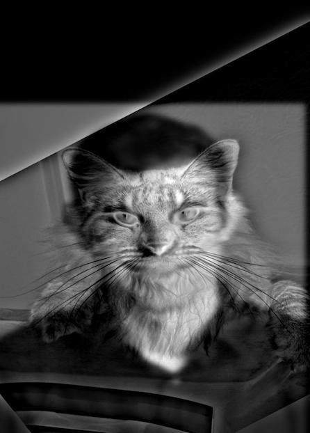
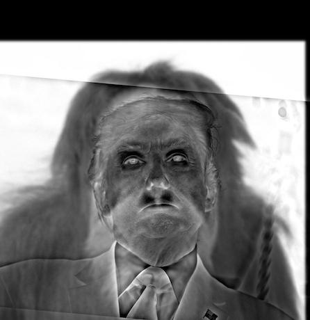
Hybrid images highlight the tendancy for human vision to resolve low-frequency information from a distance, and high-frequency information up-close. By using a low-pass gaussian filter on one image, and averaging it with a high-passed image, one can resolve one image at a distance and another up-close:

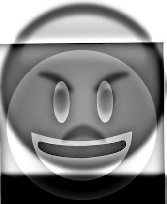
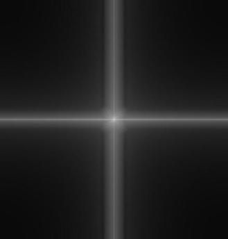
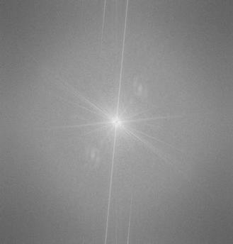
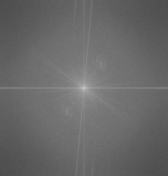
The second photo is one of an orangutan and Trump. The third example of the smiley face superimposed against the mad face emoji didn't work every well, probably because both images didn't have many low-frequency features, so even at close distances you can make out the mad emoji. The following fft plots are of the low-pass ape, the high-pass trump, and the blend respectively:

Part 1.3

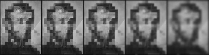
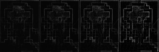
We had to construct gaussian and laplacian stacks to capture the extraction of high and low frequency features in the images. Laplacian stacks were obtained by subtracting levels in the gaussian stack.

Lincoln Gaussian Stack

Lincoln Laplacian Stack

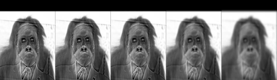
Trump_Ape Gaussian Stack

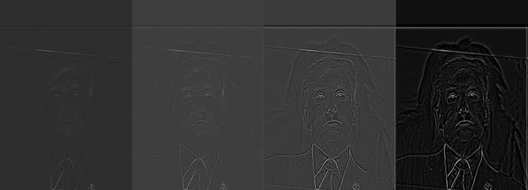
Trump_Ape Laplacian Stack

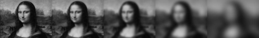
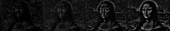
Mona Lisa Gaussian Stack

Mona Lisa Laplacian Stack

Part 1.4

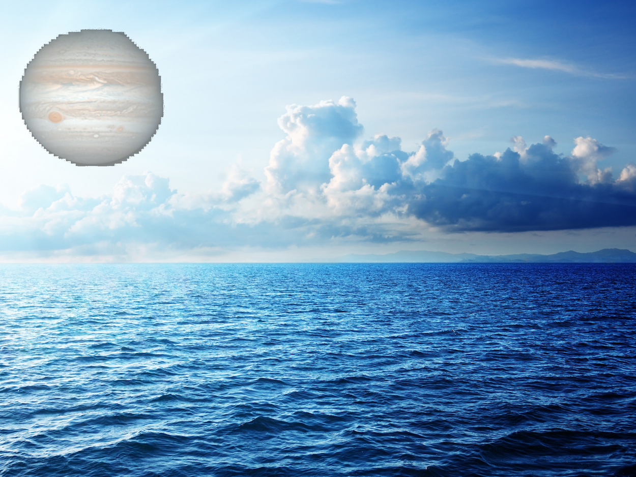
The following are some of the cool multiresolution blends that I made. The Second picture is of mars and earth blended vertically, and the third picture of jupiter and the sea, blended horizontally. The Jupiter and Sea blend didn't work very well, possibly because the sea was blended too strongly into the picture, obscuring the planet. The fourth image is of an irregular masking blend.

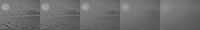
Jupiter-Sea Gaussian Stack

Jupiter-Sea Laplacian Stack

Part 2

Overview

We can achieve a better blend of two images by matching gradients and solving a least squares problem to minimize differences between the gradients of the source and target. The toy problem gives us practice with building the least squares problem, but using seperate x and y gradient constraints. Part 2.2 then implements the full gradient domain blend by using all four surrounding gradients for every pixel in the source image. Using this we can find the optimal source image pixels and paste it into the target image.

Part 2.1

Toy Problem Original:

Toy Problem Recreated:

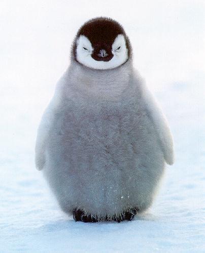
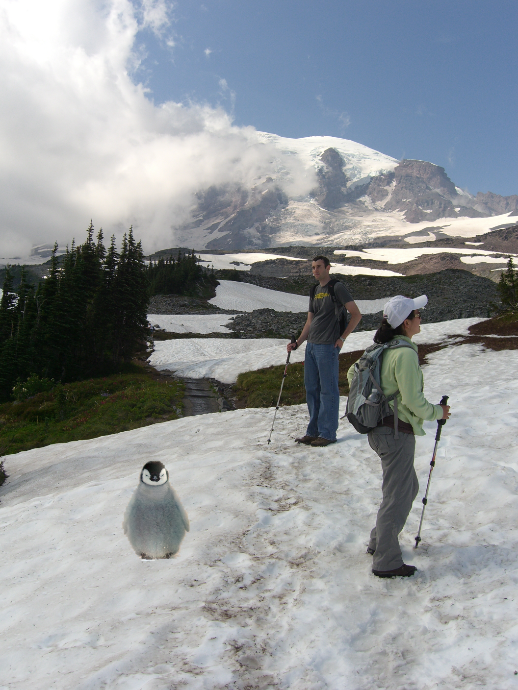
Part 2.2

To implement part 2.2, I used 4*N constraints to solve the least squares problem, where N is the total number of pixels in each image. That is, for each pixel in the image, I set a constraint that the gradient between it and one of its adjecent pixels much equal gradient of the corresponding source pixel. Since there are four adjacent pixels to every pixel (with exception to border pixels), there are 4*N constraints. 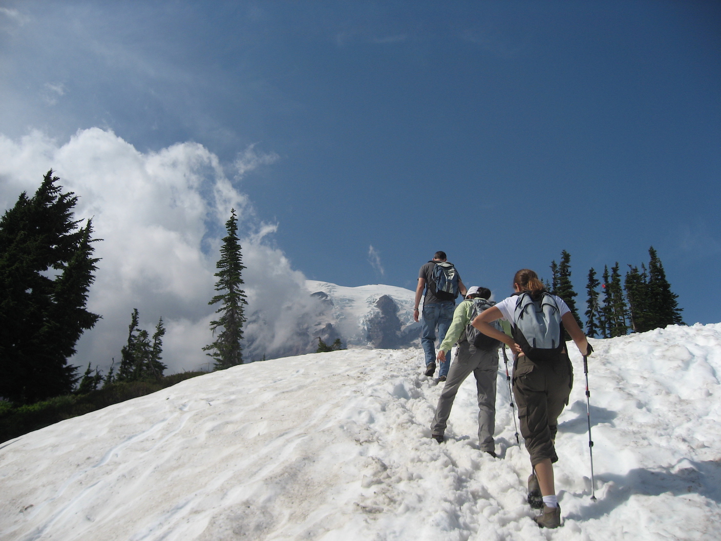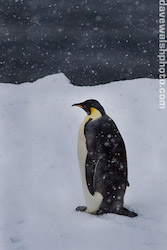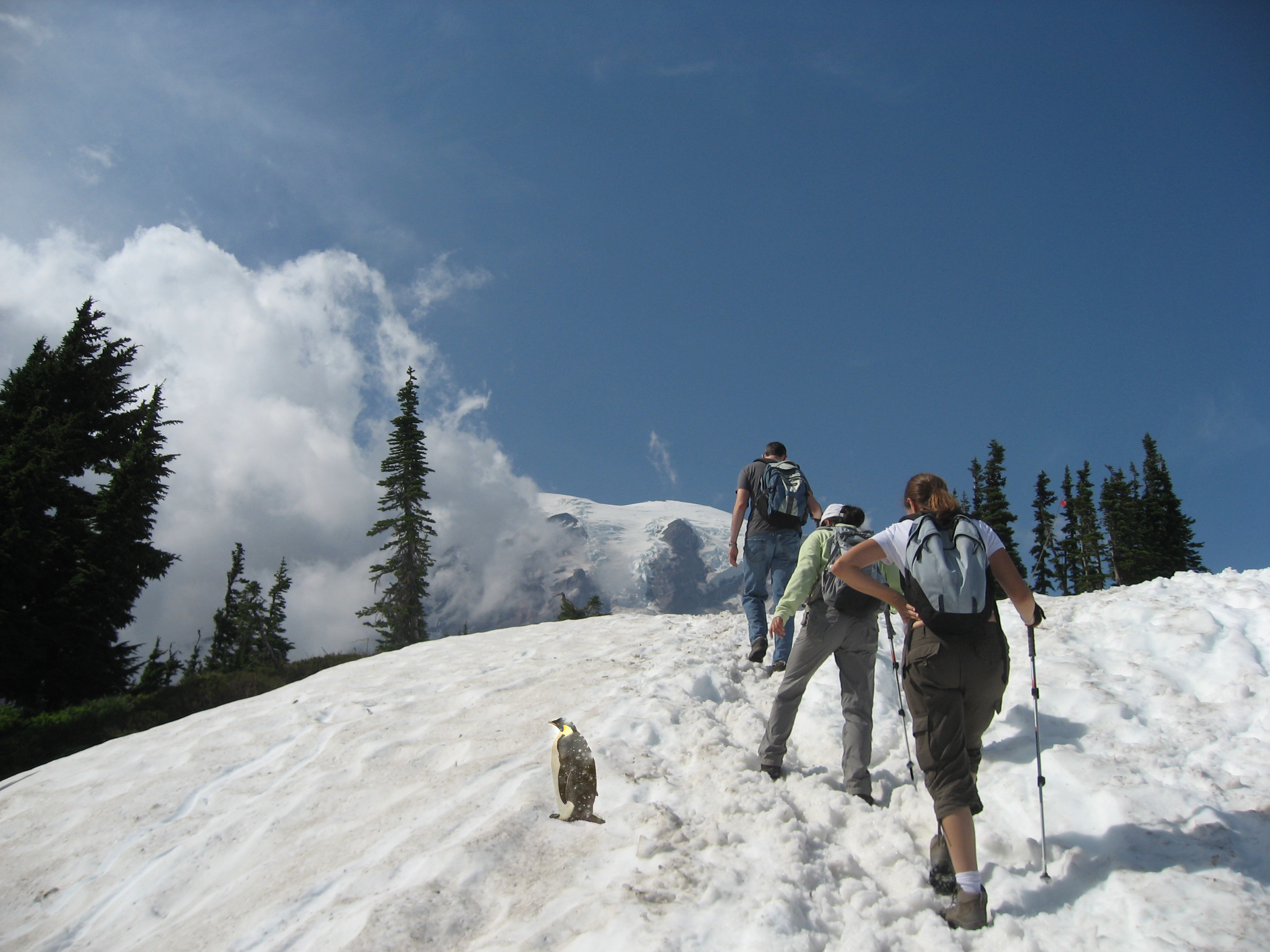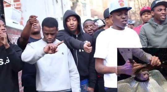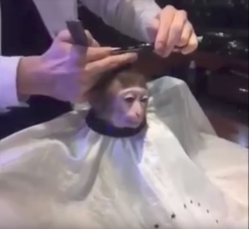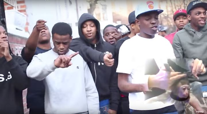Image 2: Favorite Image: Theres this internet meme of people photoshopping people cutting a monkey's hair. I wanted to see if you can use blending to get a smoother result. The first picture is the reference meme, while the bottom three are the images involved in blending. Poisson + Multiresolution Blended Comparison (Failure):

This version worked worse, and I'm not sure why.