Emailed submission on 10/9/2017, but uploaded to inst.eecs.berkeley.edu on 10/20/2017 because I got my instructional account back on 10/20/2017.
Part 1: Frequency Domain
Part 1.1: Sharpening an Image
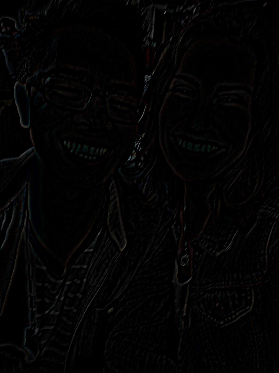
For the first part we sharpened an image using the unsharp masking technique. This involves taking a an originally blurry picture, im, getting the low pass, gaussian blurred version of the original, img, and subtracting the gaussian blurred image from the original to get the edges of the original image, im - img = imh, also known as the high pass. Then by adding the high pass filter to the original image, we get the sharpened image, ims.
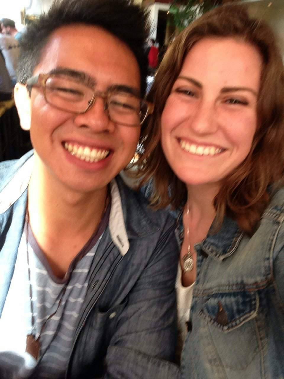 Vincent and Natasha (Original)
 |
 Guassian Blur | Low Pass Filter
 |
 Edges | High Pass Filter
 |
 Sharpened | sigma = 3 | alpha = 1
 |
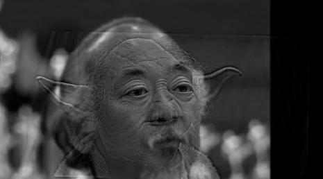
Part 1.2: Hybrid Images
As demonstrated from Part 1.1, we can can create low pass filters and high pass filters to sharpen an image. If we take the high pass filter of one image and overlay it with the low pass filter of another image. We get some interesting results. I added one colored one for the Bells & Whistles to demonstrate that colored hybrid images are harder to look good, but with the right pair of images, it can still produce something nice.
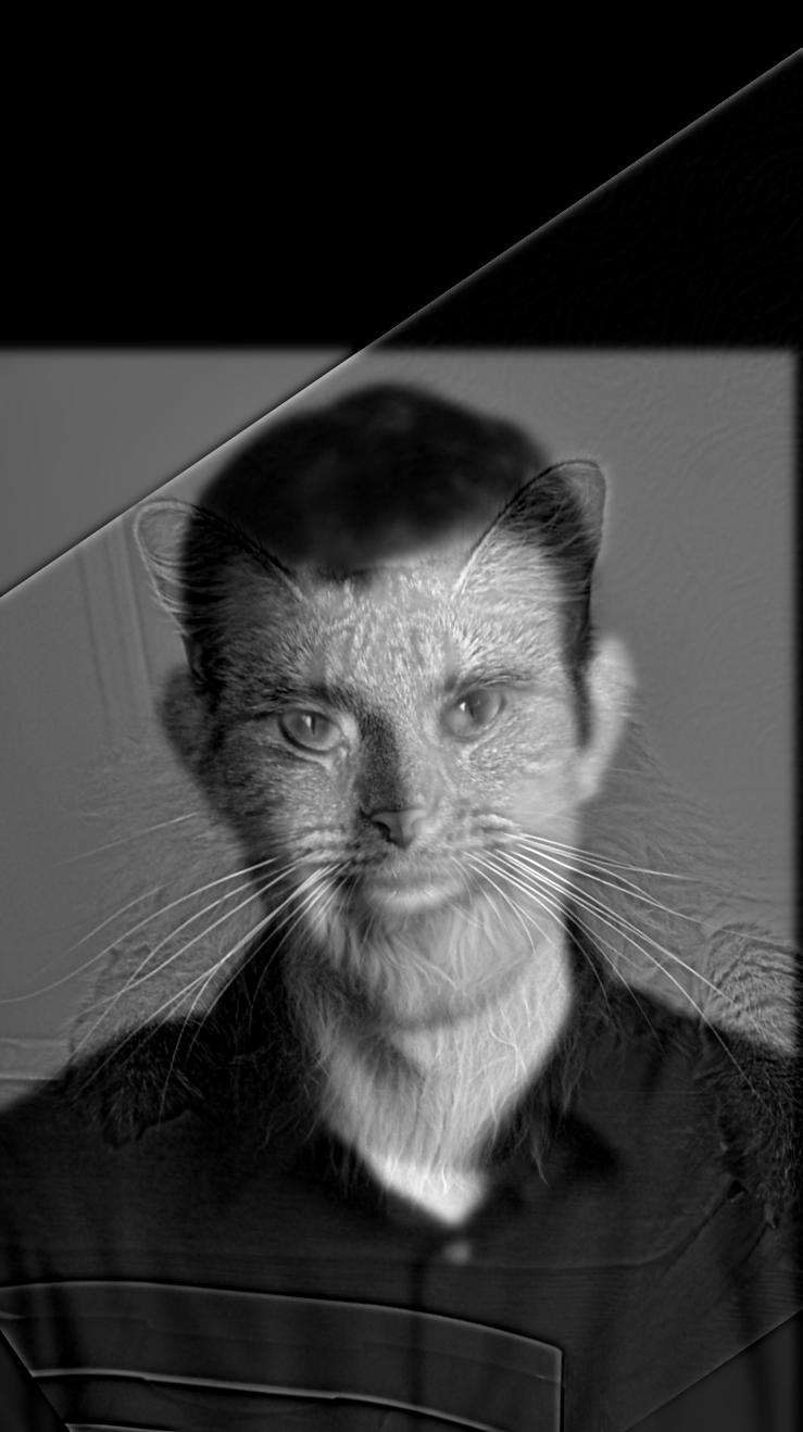 Catman
 |
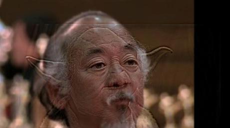 Mr. Yoda Miyagi
 |
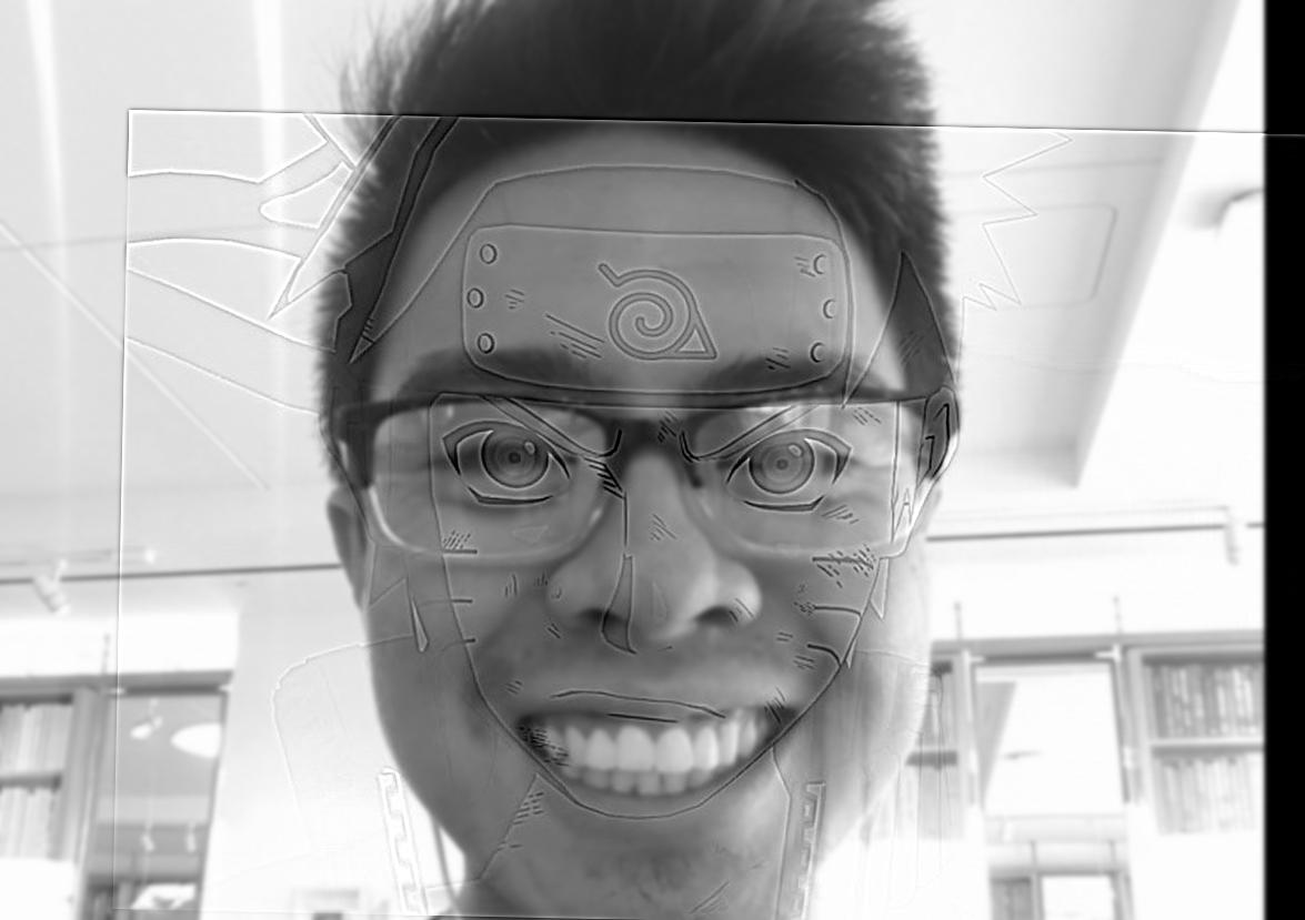 Naruto Escueta
 |
 Belle and Natasha (failure)
 |
Fourier Transforms
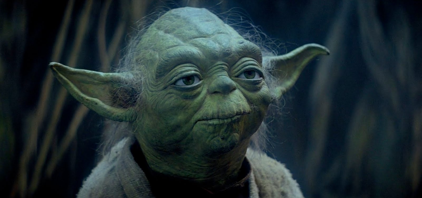 Yoda
Yoda |
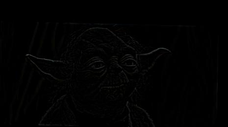 Yoda High Pass
 |
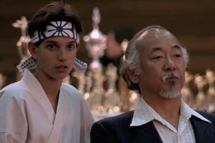 Mr. Miyagi
 |
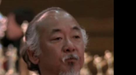 Mr. Miyagi Low Pass
 |
 Mr. Yoda Miyagi
 |
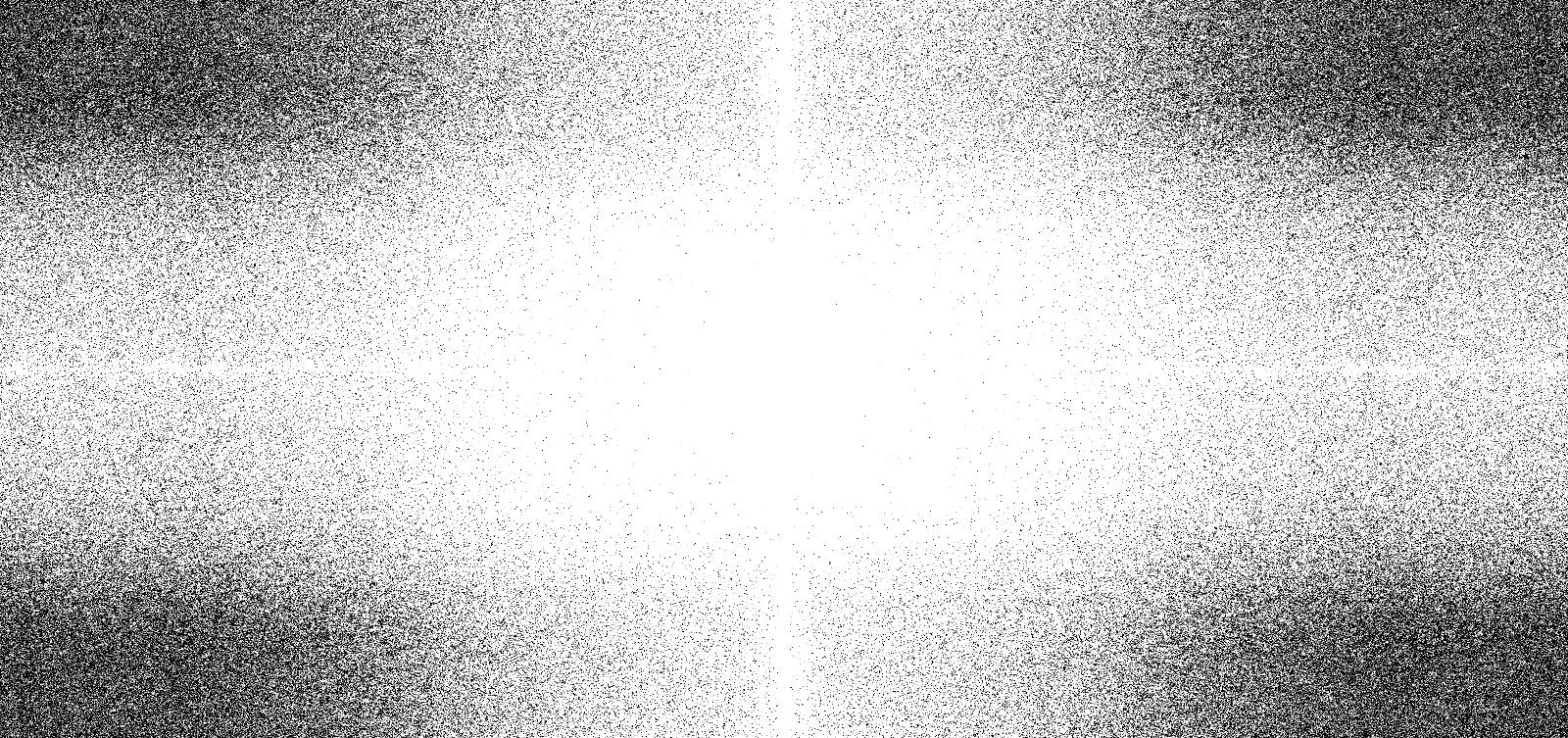 Yoda Fourier
 |
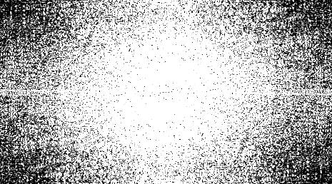 Yoda High Pass Fourier
 |
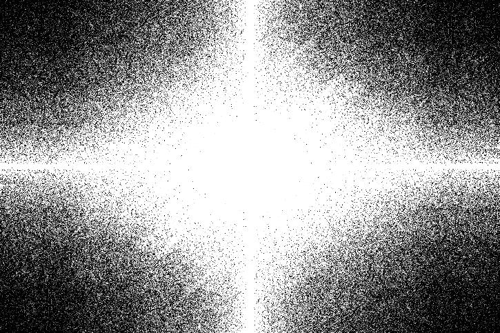 Mr. Miyagi Fourier
 |
 Mr. Miyagi Low Pass Fourier
 |
 Mr. Yoda Miyagi Fourier
 |
1.3 Gaussian and Laplacian Stacks
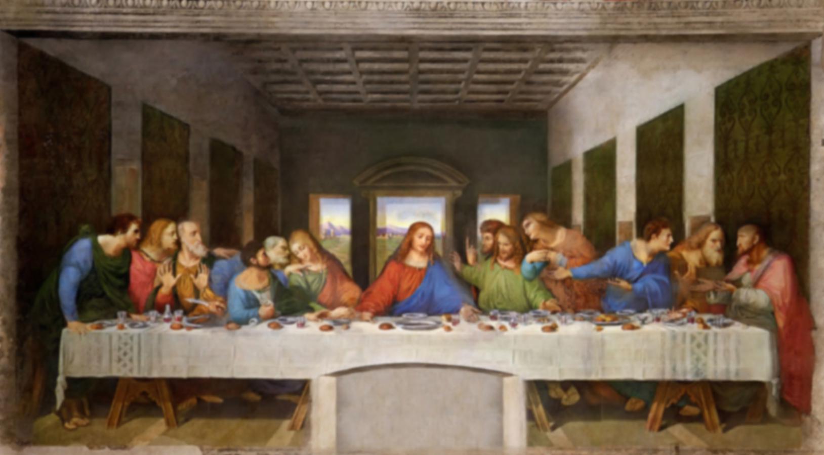
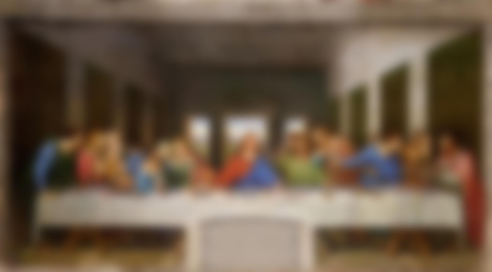
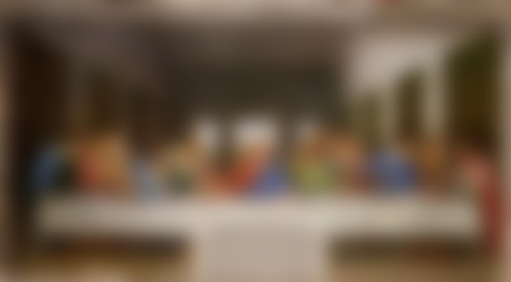
Next we implemented Gaussian and Laplacian Stacks. A Gaussian Stack is a series of low pass images with increasing Gaussian blurs. My examples do sigma of 2, 4, 8, 16, 32. A Laplacian Stack is a series of high pass images that is a low pass image minus the gaussian with a sigma one power higher. Below are some examples of that. One is of Leonardo da Vinci's The Last Supper. I used this because of the depth and sharp lines offered. And I used the blurriest low pass filter and the laplacian stack to rebuilt the image. The other is one of my failure image, Belle and Natasha. The reason I used this is because Belle's lines are so sharp that it's interesting how the stacks slowly make Belle fade away and only Natasha is left by sigma = 16.
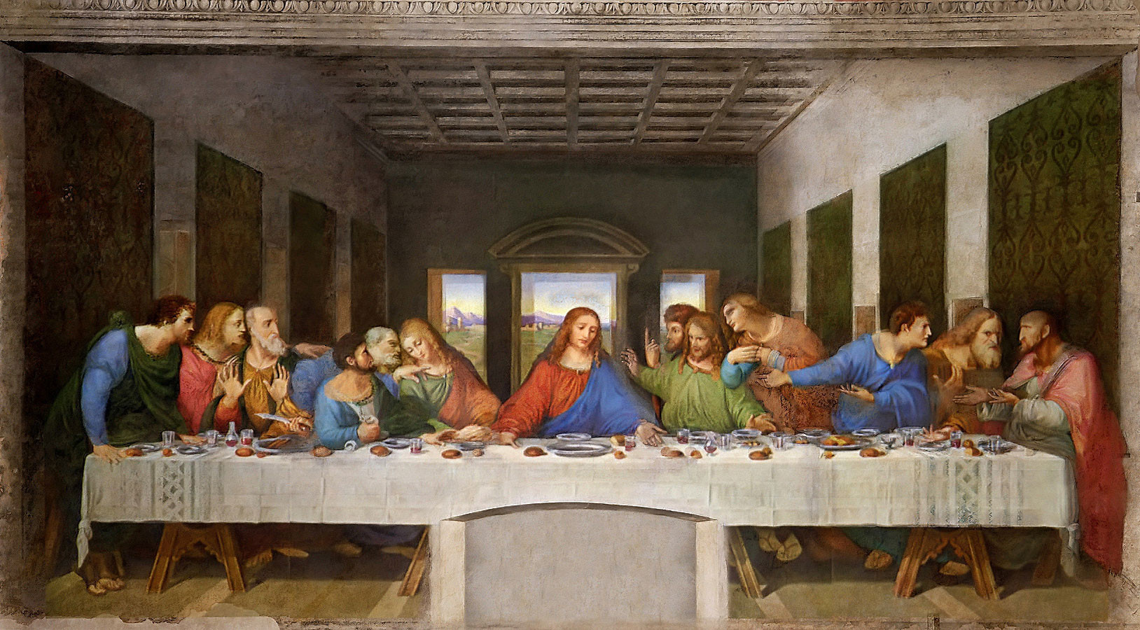 Original The Last Supper
 |
 Rebuilt
 |
 Gaussian (sigma=2)
 |
 Laplacian (sigma=2)
 |
 Gaussian (sigma=4)
 |
 Laplacian (sigma=4)
 |
 Gaussian (sigma=8)
 |
 Laplacian (sigma=8)
 |
 Gaussian (sigma=16)
 |
 Laplacian (sigma=16)
 |
 Gaussian (sigma=32)
 |
 Laplacian (sigma=32)
 |
|
Original |
 Gaussian (sigma=2)
 |
 Laplacian s(igma=2)
 |
 Gaussian (sigma=4)
 |
 Laplacian (sigma=4)
 |
 Gaussian (sigma=8)
 |
 Laplacian (sigma=8)
 |
 Gaussian (sigma=16)
 |
 Laplacian (sigma=16)
 |
 Gaussian (sigma=32)
 |
 Laplacian (sigma=32)
 |
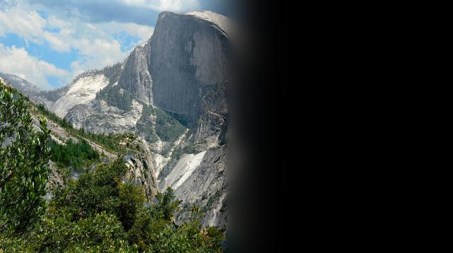
Part 1.4: Multiresolution Blending
Successfully implemented multiresolution blending by doing something very similar to rebuilting The Last Supper from stacks. Given 2 images, im1 and im2, and given a mask filter mask. First we made a negative version of our mask, giving us mask and neg_mask We made Laplacian and Gaussian stacks for each image and each mask.
We made the first portion of our final photo by taking each high pass filter in the Laplacian stack of im1 and multiplying it by the Gaussian of mask with similar sigmas. Afterward, we add all those results together and add it to the our blurriest gaussian in the stack of im1 which is multiplied by the blurriest mask Gaussian. Then repeat this with im2 and neg_mask and we end up with the photos we see below.
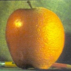 Oraple (Apple and Orange
 |
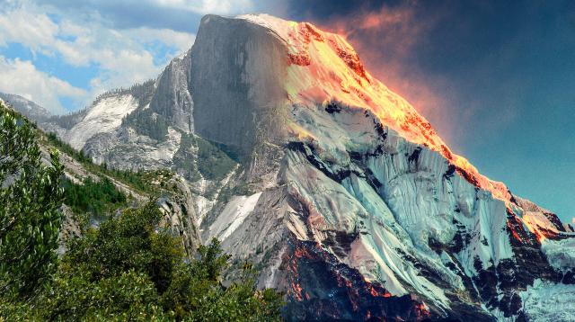
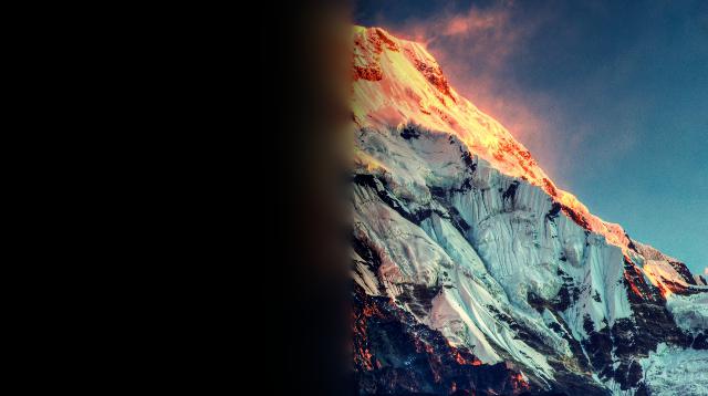
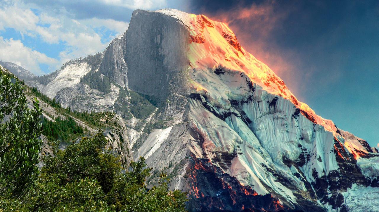 Half Everest (Half Dome and Mt. Everest)
 |
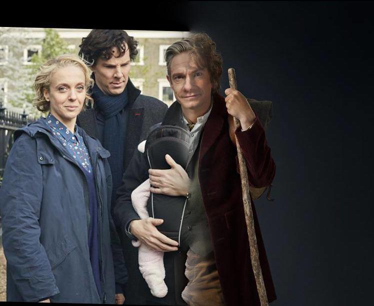 Martin Freeman (Watson and Bilbo Baggins)
 |
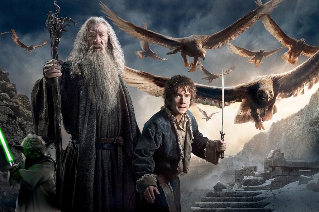
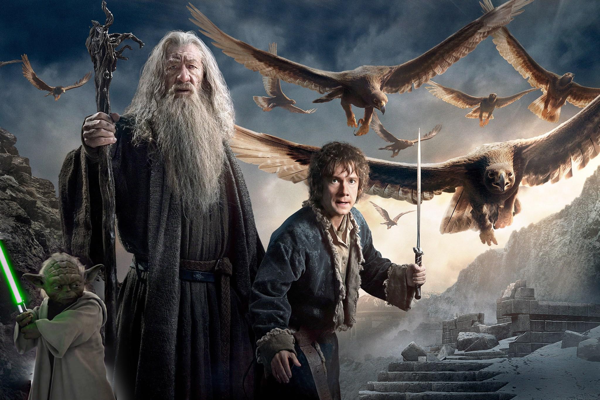 Masters (Yoda and Gandalf)
 |
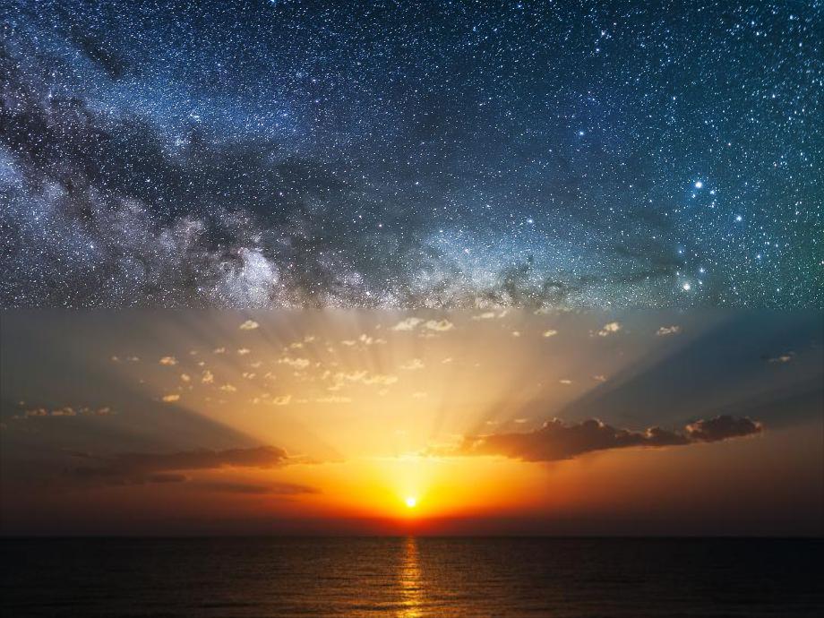 The Sky (Sunrise and Starry Night)
 |
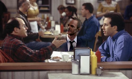
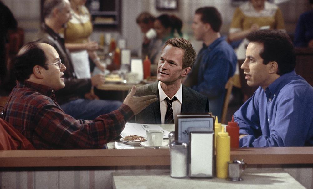 Legendary Art Vandalay (Jerry, George and Barney)
 |
This is the deconstruction of the process stated above. The ssum of all the center images form the finall middle image shown below. The center images are the addition of the left and right adjacent to it.
 Left
Left |
 Laplacian (sigma = 32)
 |
 Right
Right |
 Left
Left |
 Laplacian (sigma = 16)
 |
 Right
Right |
 Left
Left |
 Laplacian (sigma = 8)
 |
 Right
Right |
 Left
Left |
 Laplacian (sigma = 4)
 |
 Right
Right |
 Left
Left |
 Laplacian (sigma = 2)
 |
 Right
Right |
 Left
Left |
 Gaussian (sigma = 32)
 |
 Right
Right |
Part 2: Gradient Domain Fushion
The goal of this section of the project was to blend one image on top of another without the image placed doesn't look out of place. We do this by playing with gradients to not change anything within the traget image, only change things with the source image. We no longer will look at intensities or Laplacian blending, but use the gradients of a source image and the original target image along with the least squares problem to do Poisson blending.
Part 2.1: Toy Problem
The toy problem involved constructing an image, im given a matrix A and an image b. To get A we contruct a (l * w) x (l * w) sized array where each row corresponds to a final pixel value represented by all elements of the original image. If a pixel is at an edge, we just put 1 on the corresponding row and column index where the pixel would belong in a 2d image. Otherwise, we place a 4 on the corresponding row and column index where the pixel would belong in a 2d image and -1 on the row and column index that would be adjacent to the pixel that we placed a 4 on the 2d array. By deconstructing im into a 1d array, 1d_im of size l * w from its 2d array we can do A.dot(1d_im) to get b. Then if we constructed the equation (Ax - b)^2 = 0, we would solve for x to get the 1d version of the reconstructed image. By reshaping it, we get the reconstruction as shown below.
 Original
 |
 Reconstructed
 |
Part 2.2: Poisson Blending
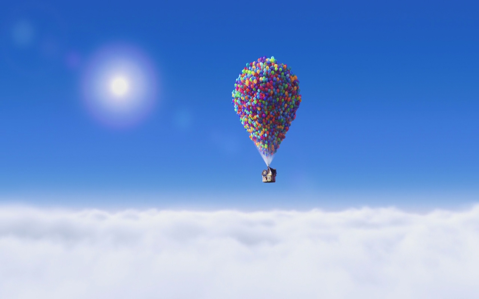
For this part of the project, we wanted to blend in a source picture, sim, to a target picture, tim, when given a mask that indicates where sim goes. The way we did that was very similar to the toy problem. By getting the portion of the source image we want through applying the mask, we apply the Laplacian filter over it to create a gradient. Next, we would surround the image with a portion of the target image. Afterward, we use a least squares solver with the current image we have with a matrix, A to get a manipulated image where sim is meant to blend into tim naturally. Our matrix A is an invertible matrix with 1 on the diagnoal if the pixel at that index is meant for a pixel of the target image and a flattened Laplacian pyramid where the corresponding pixel to that row is part of the source image. Below is the house from UP, sim, being applied to a scene in Finding Dory tim. Below that are other results including one failure.
 Source
 |
 Target
 |
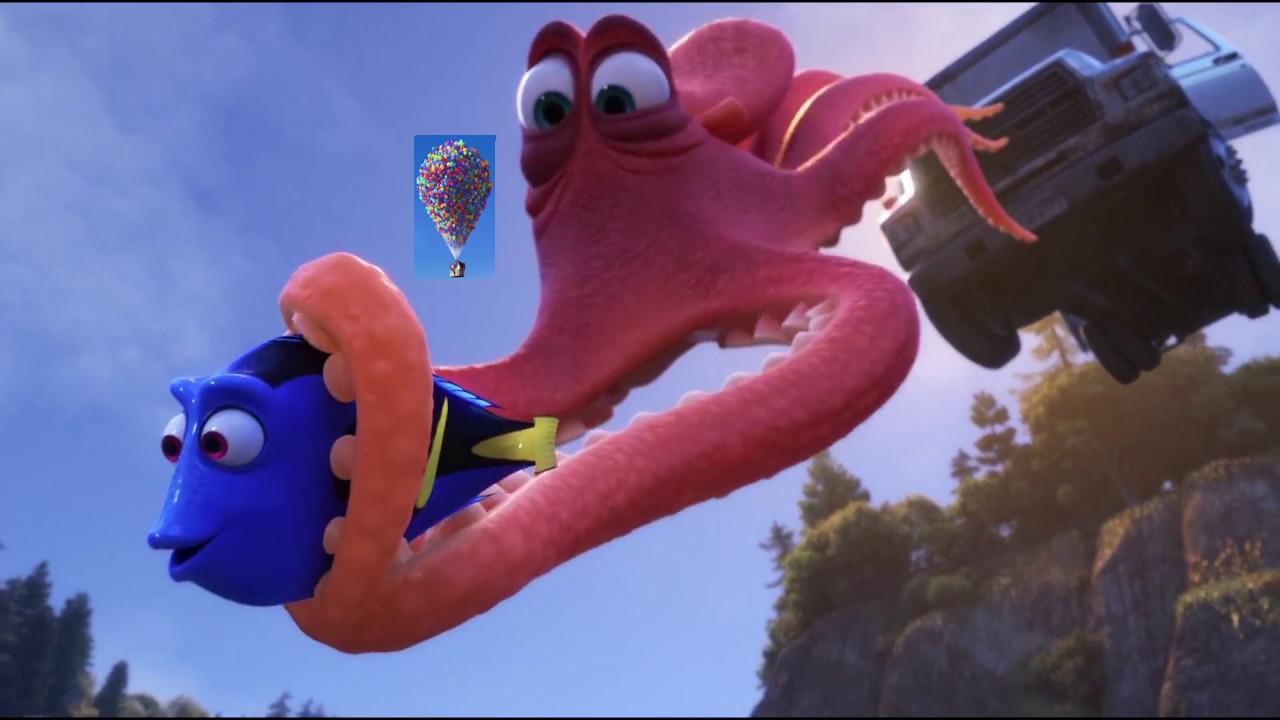 Overlayed
 |
 Blended
 |
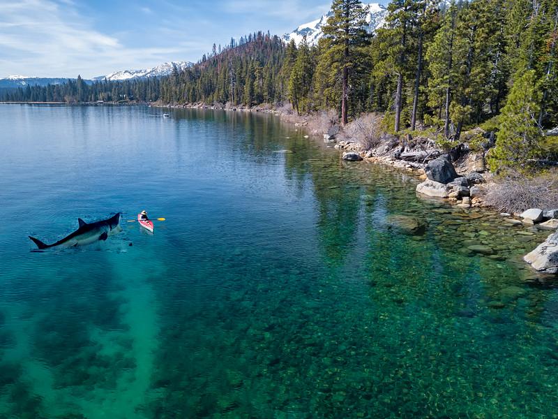 Failure (because background of source very different than source)
 |
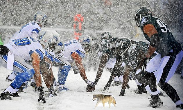 Footballers dances with wolves
 |
|
Pixarception |
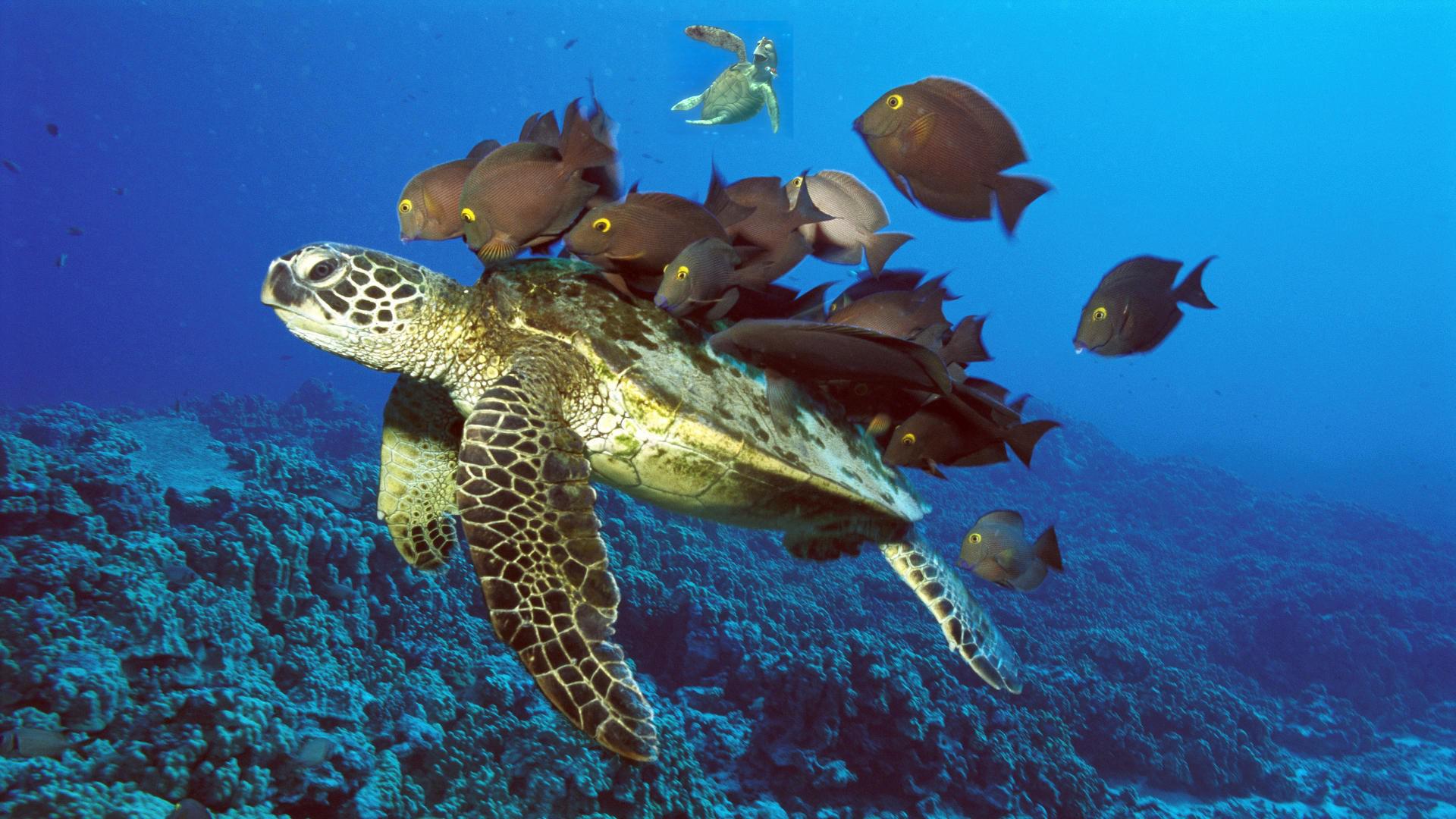 Real meets animated
 |
The pictures below show the difference between Laplacian blending and Poisson blending. The Seinfled shows pros and cons of both blends. The Laplacian blending allowed Barney to seem fully there, but George's hand started to fade into the suit. The Poisson blend didn't go well because the mask was small and made it so Barney faded into the environment. However, the small section that wasn't faded allows the suit to have a similar color to the image itself.
The Yoda and Hobbit image shows how the Laplacian blending allowed Yoda to be fully in the sccene, but part of his robe began to blend a little to the background emitting white pixels. The Poisson blending didn't allow Yoda to blend so well. This is because Yoda is light while the background was dark. So Yoda blended into the background and beacame dark and hard to see.
Overall, it seems that Poisson blending works when you want to blend two similar pictures int terms of the content of the iamge, but are slightly different colors. Laplacian blending works better when you want to blend two images that are similar in color.
|
Laplacian blending |
 Poisson blending
 |
|
Laplacian blending |
 Poisson blending
 |