CS194-26 Project 3

Project Overview

The goal of this project was to manipulate images using gradients and frequencies. For part 1, by using Gaussian and Laplacian representations of my images, I can generate sharpened images, hybrid images (that show different objects at different distances), and seamlessly blend objects. For part 2, I improved seamless blending using the poisson blending technique to calculate gradients.

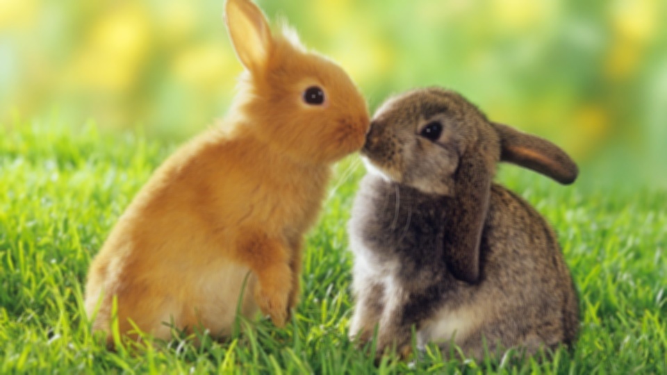
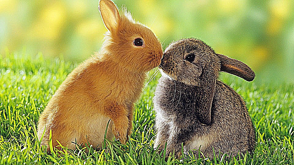
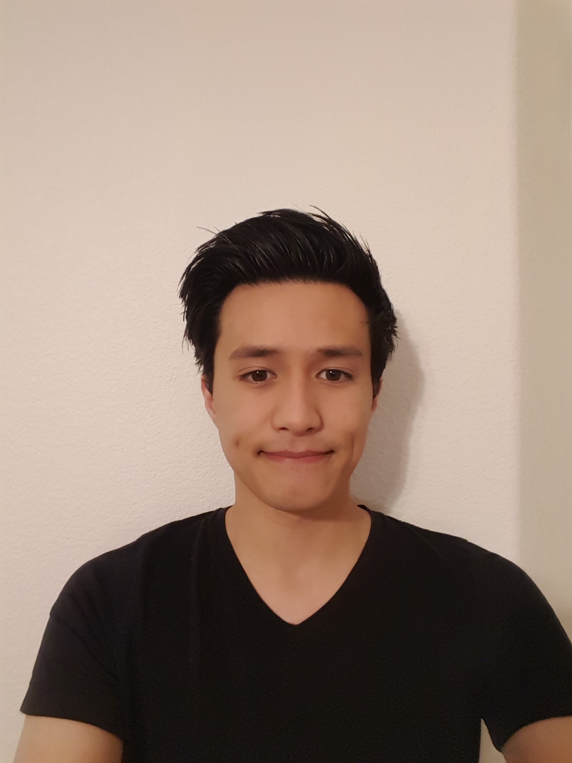
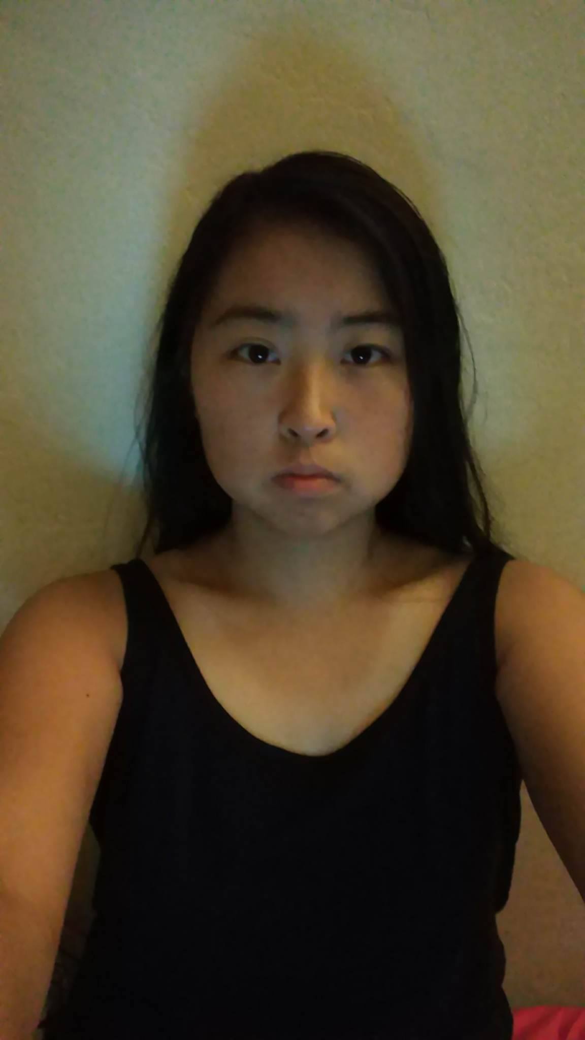
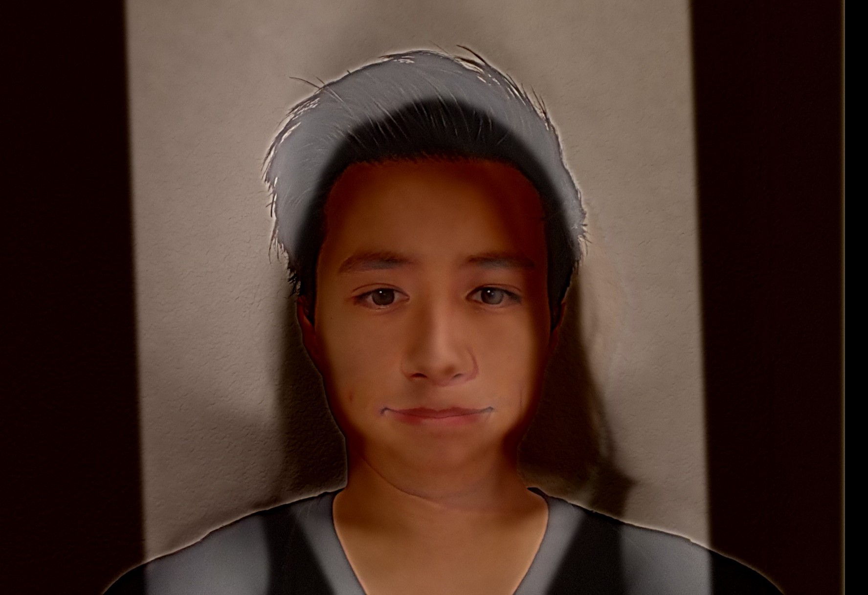
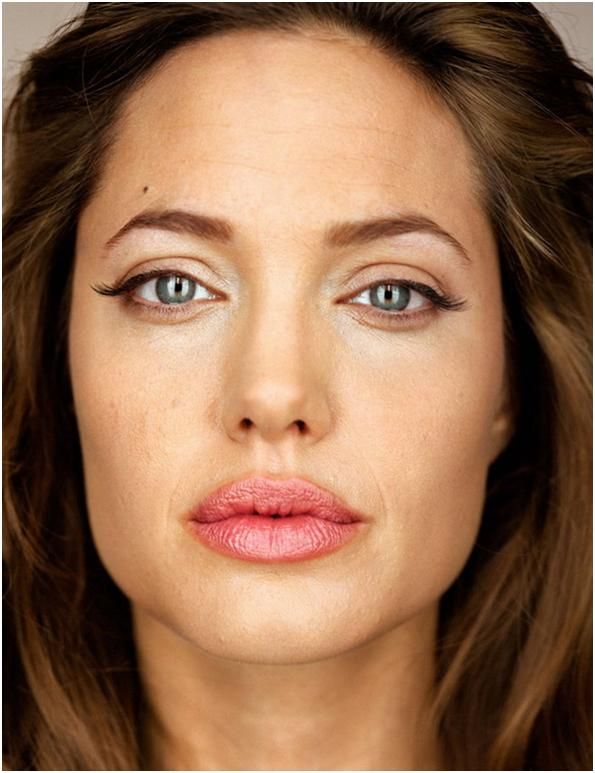
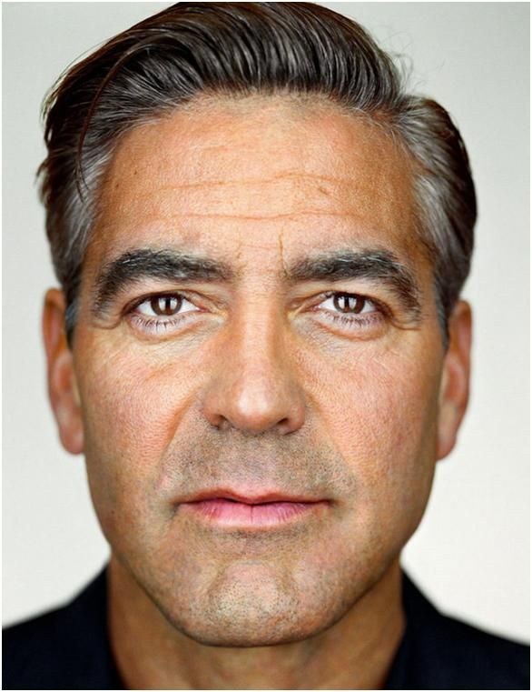
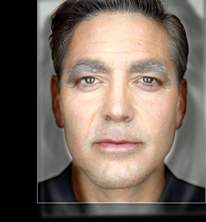
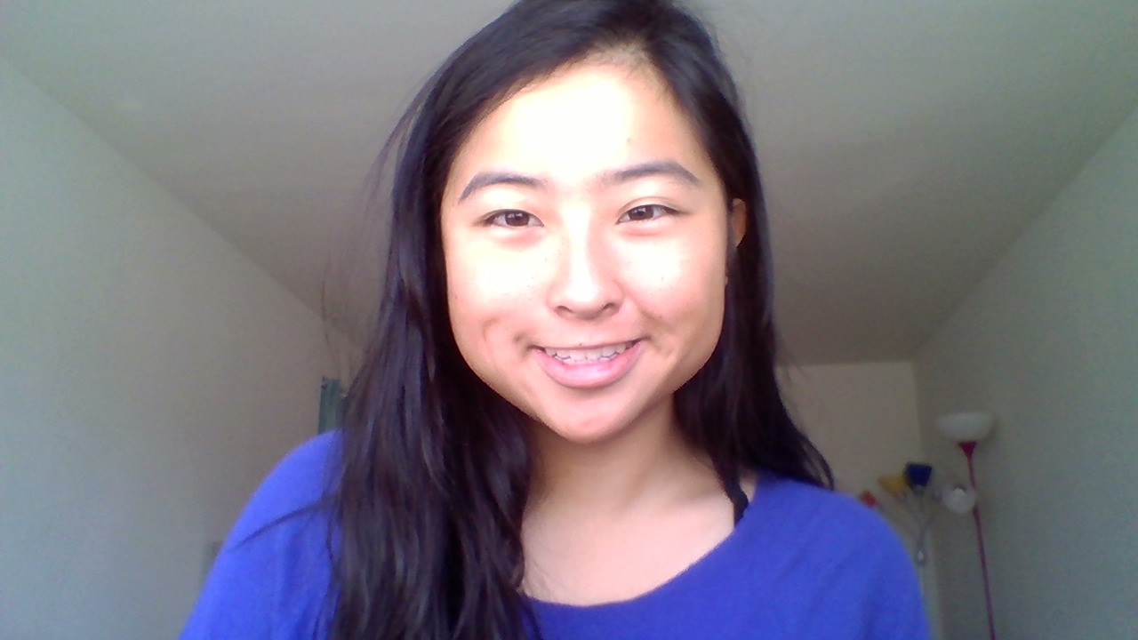
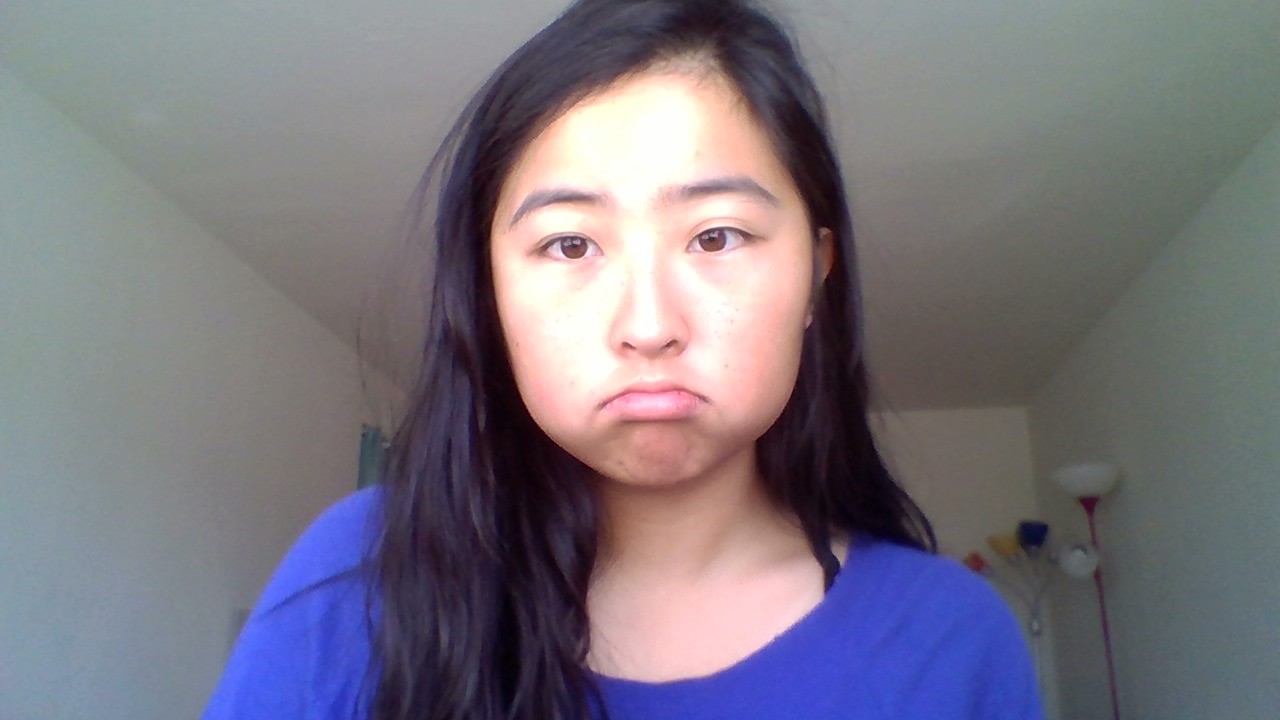
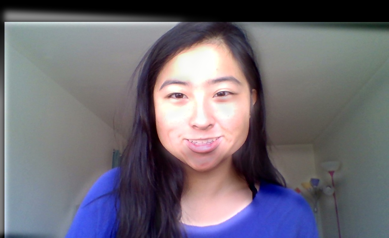
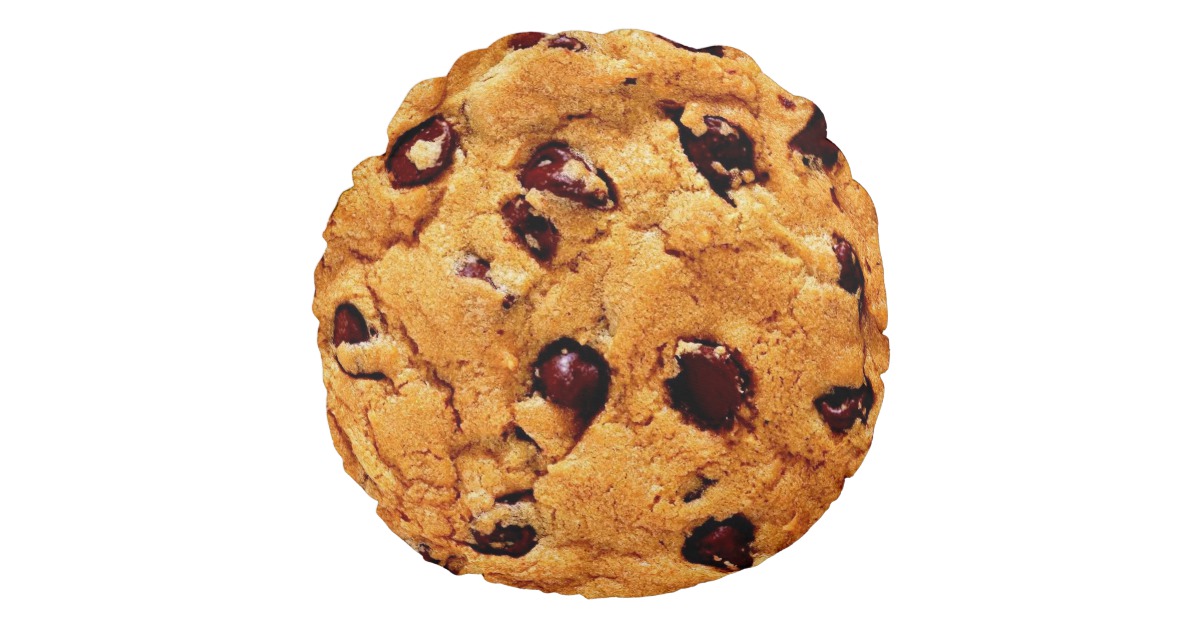
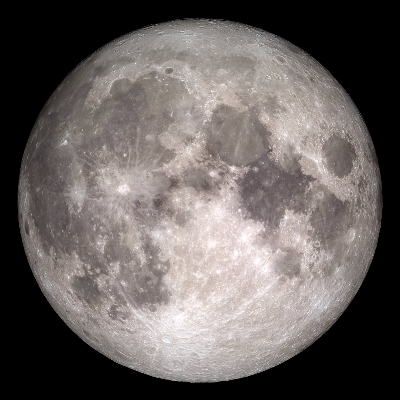
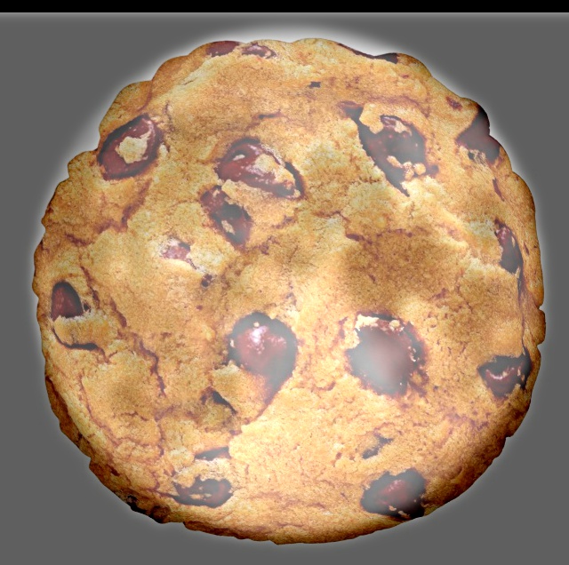
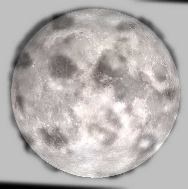
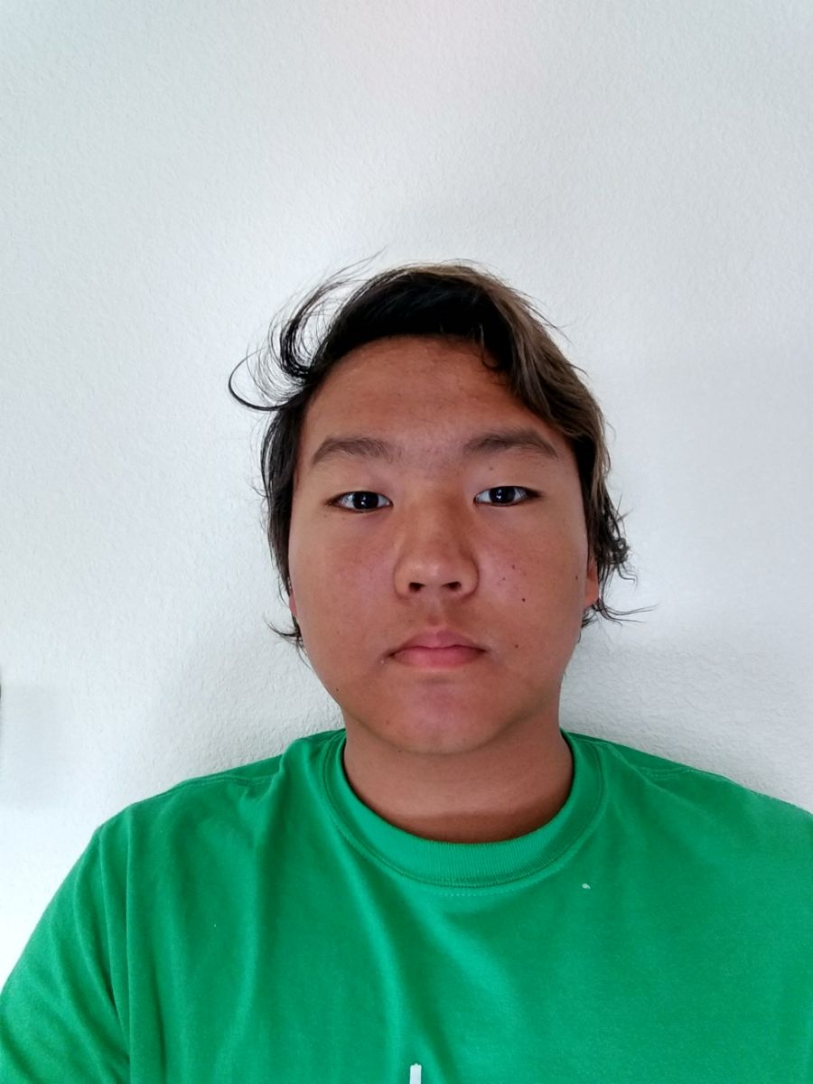
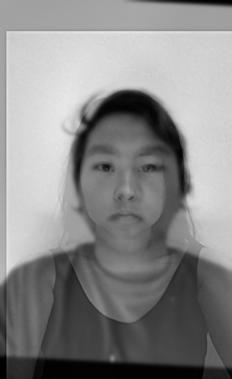
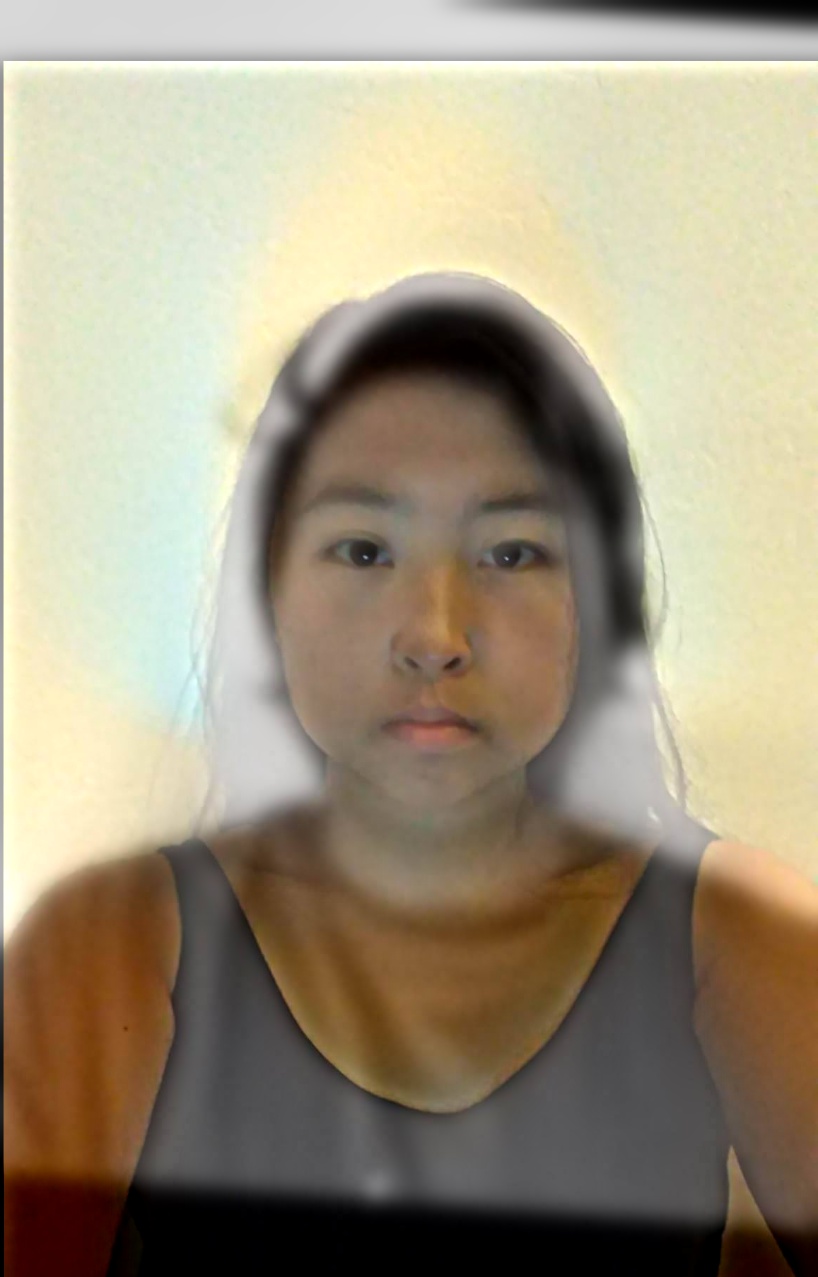
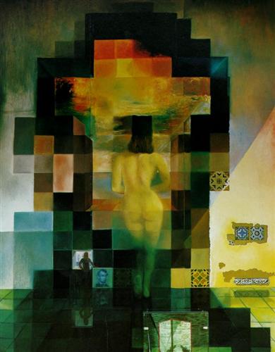
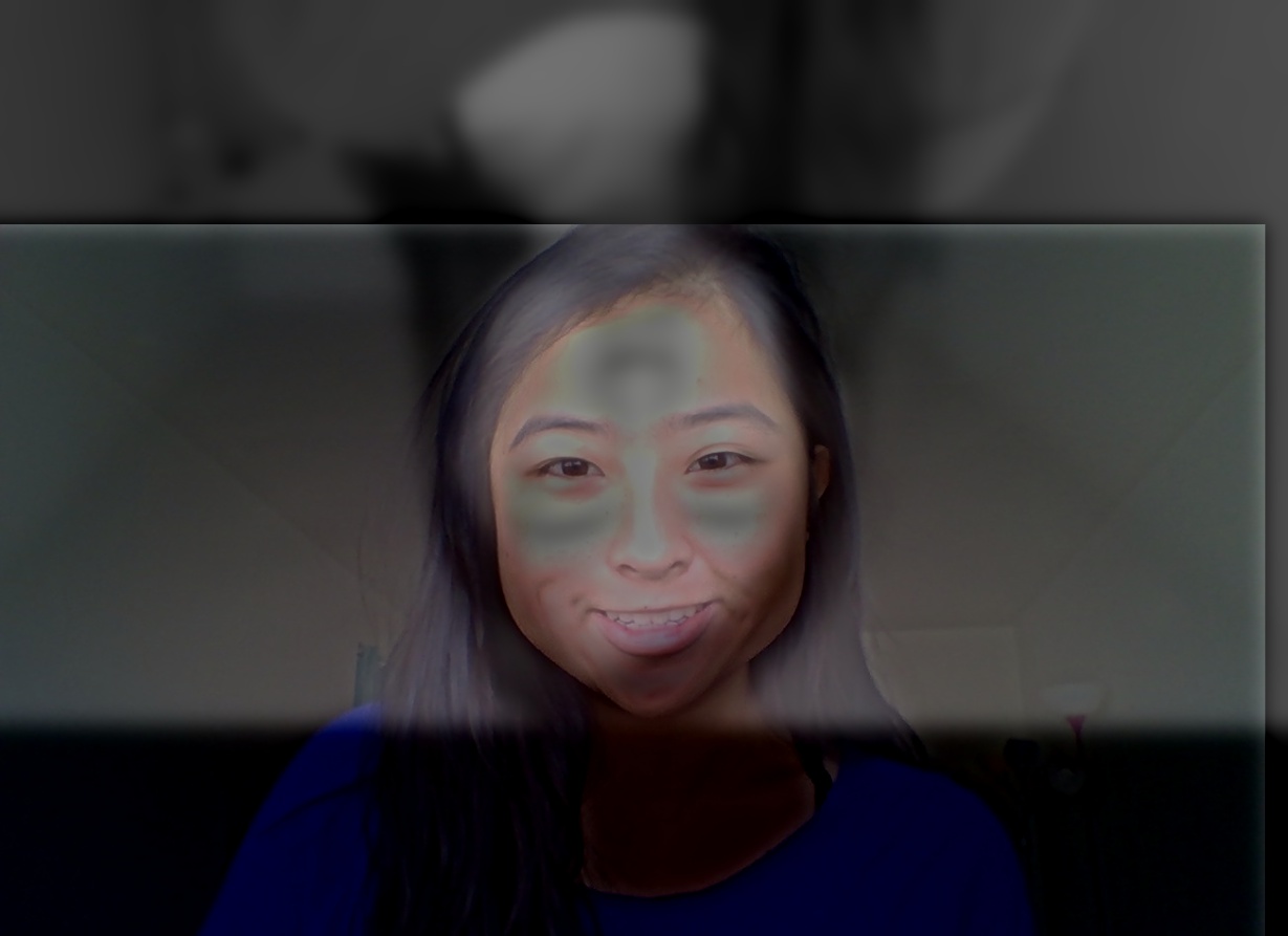
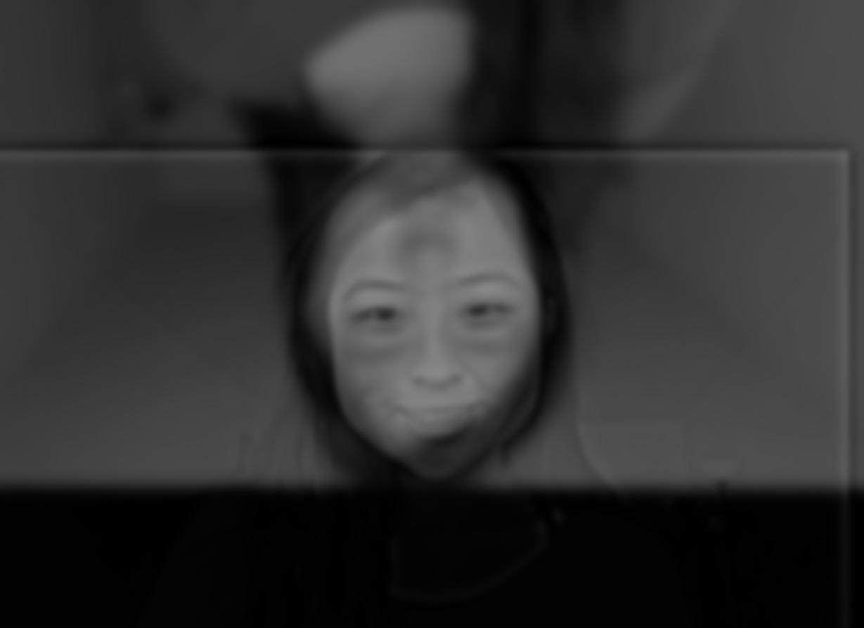
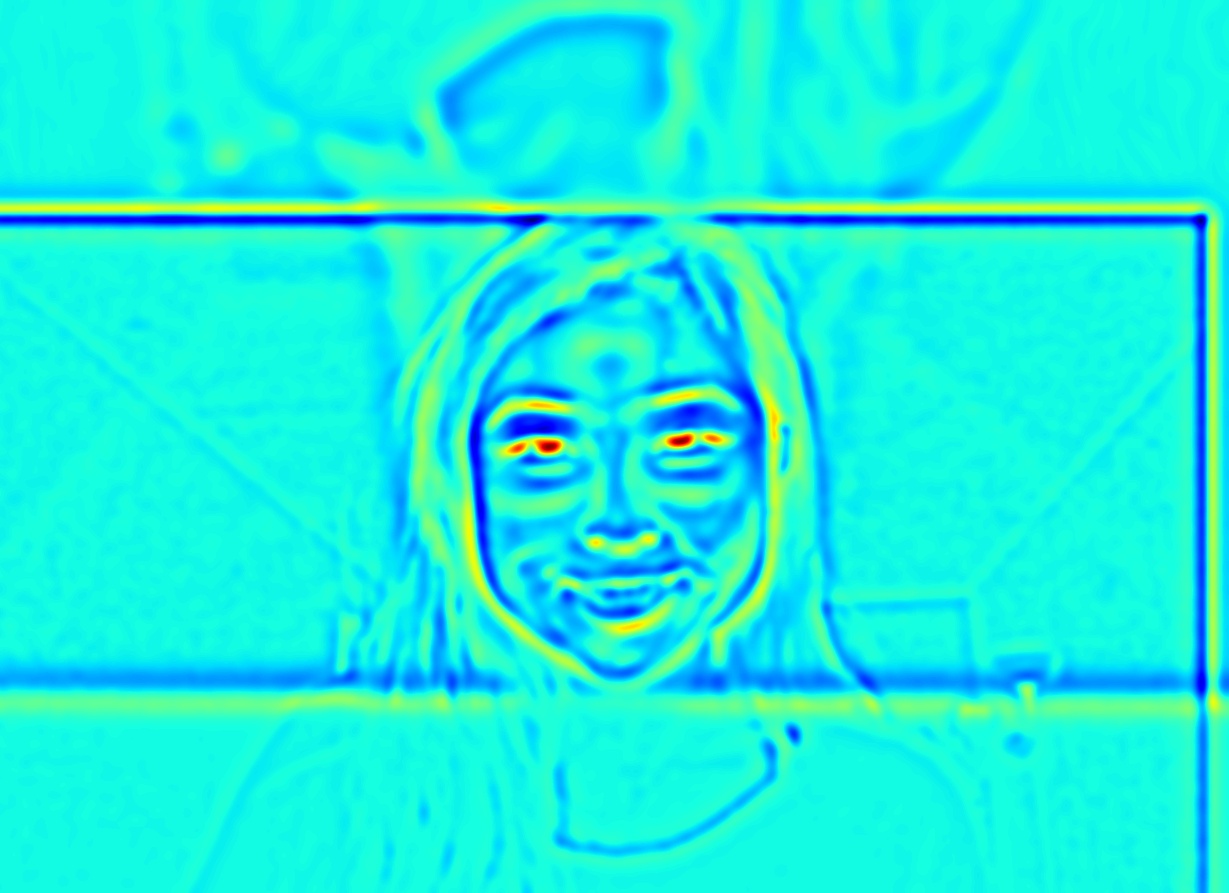
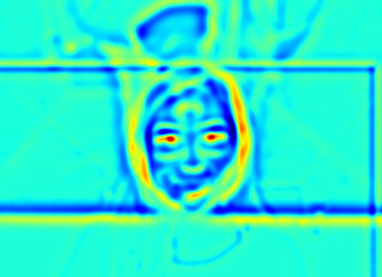
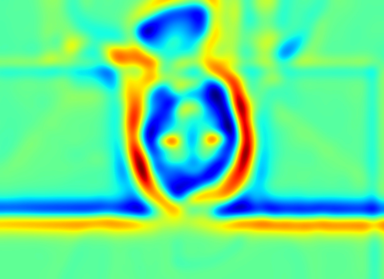
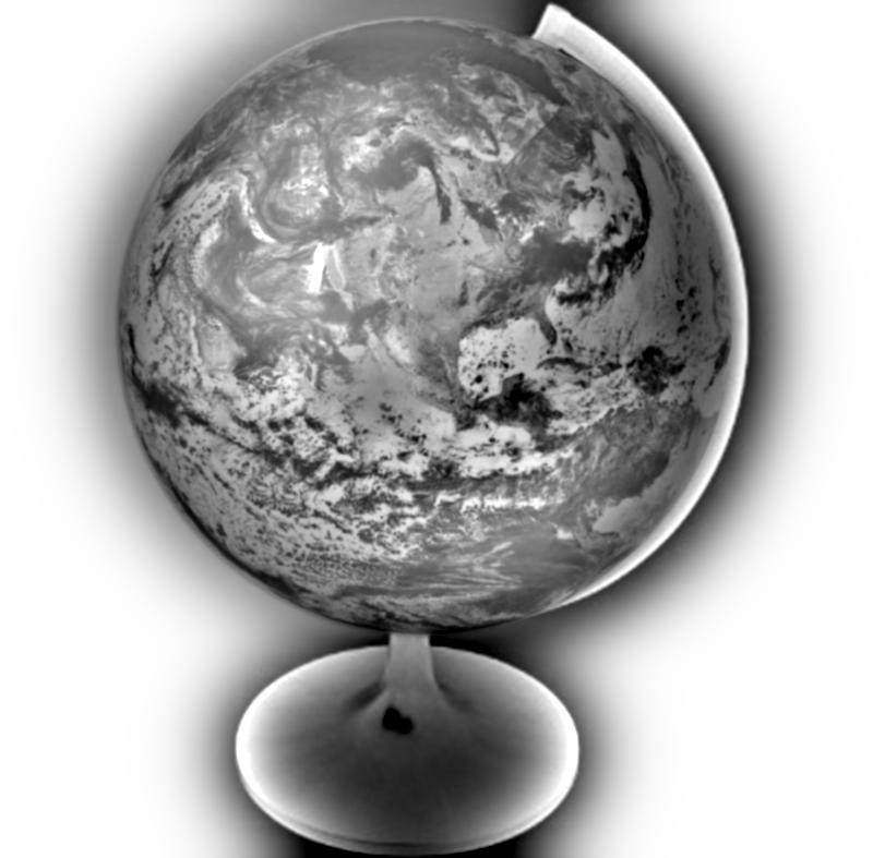
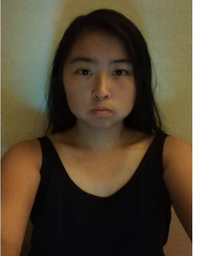
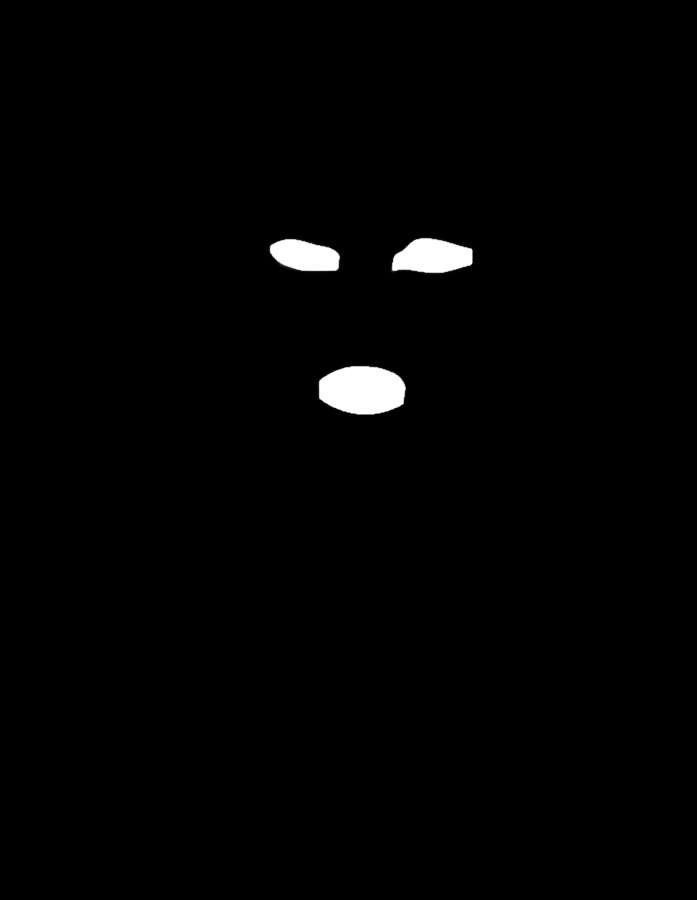
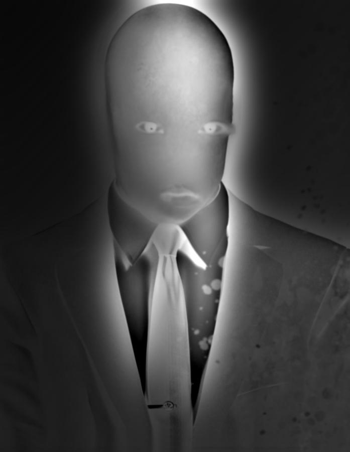
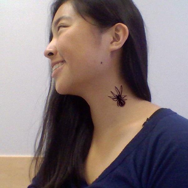
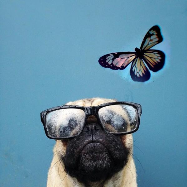
1.1: Sharpening with an Unsharp Mask

Method

To sharpen an image:

1. Compute the image's gaussian resulting in a lowpass version of the image
2. Subtract the low frequency image from the input image to get the high frequency:
   high_frequency = input - low_frequency
3. Sum the high_frequency and the input image weighted by α (which determines image sharpness). I needed to compute a weighted sum where the images summed to 1 (otherwise the photo was too dark or contained artifacts).
   output = α * input + (1-α) * laplacian

Results

1.2:Hybrid Images

This section was implemented using the SIGGRAPH 2006 paper on creating static images that appear to show different subjects depending on the viewer's distance. When viewing images at a distance, the eye perceives low-frequency information. When closer, the eye is able to detect the high-frequency details.

Method

1. Input 2 images: A, B.
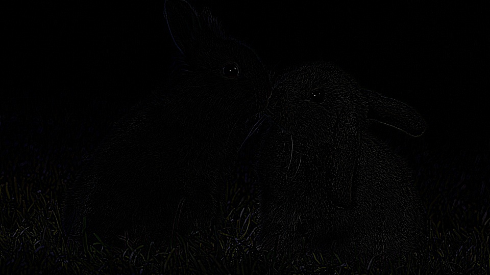
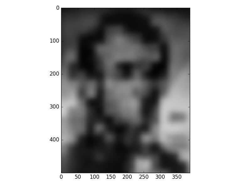
2. Compute high frequency image A (technique described in previous section)
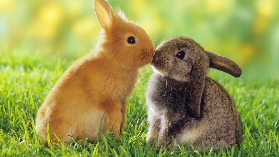
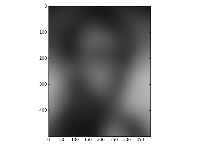
3. Compute low frequency image B
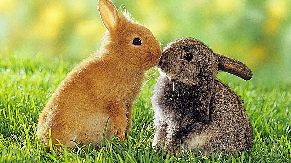
4. Average two images

Results

1.3: Gaussian and Laplacian Stacks

Gaussian and laplacian stacks are collections of the same image (of the same size) with incremental filtering on top. For example, gaussian stack will start with the input image.

Method

1. Input image A with desired stack level d
2. G_1(A) = Gaussian(A)
3. For i in 1...d: G_i(A) = Gaussian(G_{i-1}(A))
4. L_1(A) = A - G_1(A)
5. For i in 1...d: L_i(A) = G_i(A) - (G_{i-1}(A))

Results

Lincoln Analysis

Gaussian Stack and Laplacian Stack

Topsy Turvy: Upside down?

Multiresolution Blending

Often we see images that seem like they can't be real... Well, with seamless blending, you can manipulate images to blend two different images together to appear as if they're one. Multiresolution blending takes in two images you want to blend as well as a binary (black/white) mask that will specify which parts of an image you want to keep. Procedure:

1. Read in images (A, B) and a mask as grayscale
2. Compute Gaussian and Laplacian stacks for all 3 images (stacks generated with depth=5)
3. For each level d of the stack:
   L_i(AB) = G_i(M)*L_i(A) + (1-G_i(M)) * L_i(B)
4. Calculate the Gaussian for level (d+1) of the images and the mask
   outputGaussian = G_{d+1}(M) x G_{d+1}(A) + (1-G_{d+1}(M)) x G_{d+1}{B}
5. The final result is the sum of the result laplacians calculated in step 3 and our outputGaussian

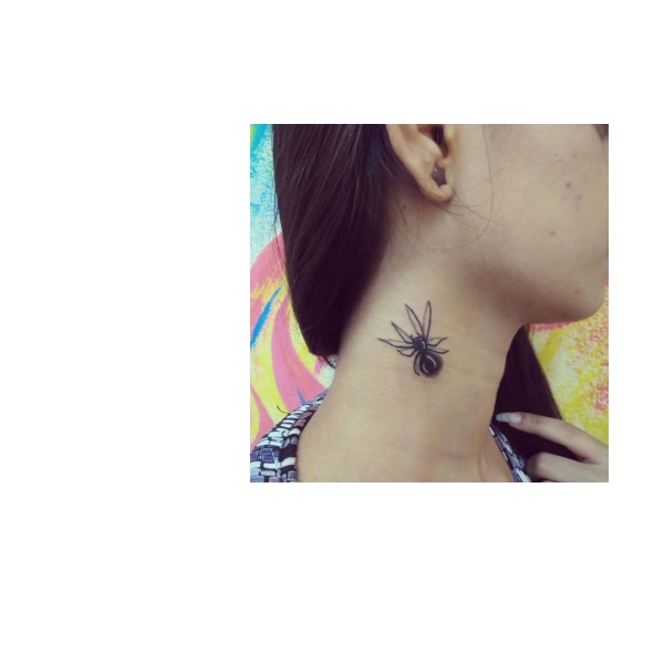
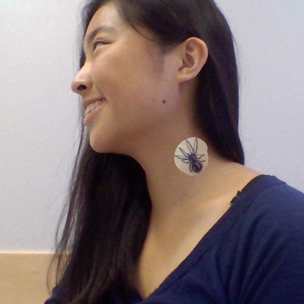
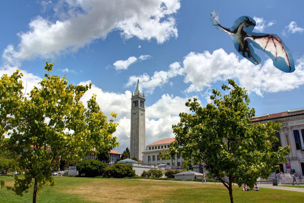
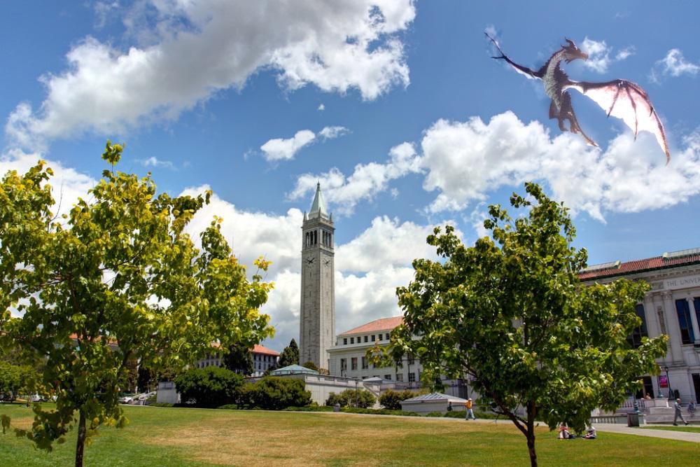
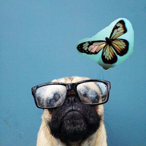
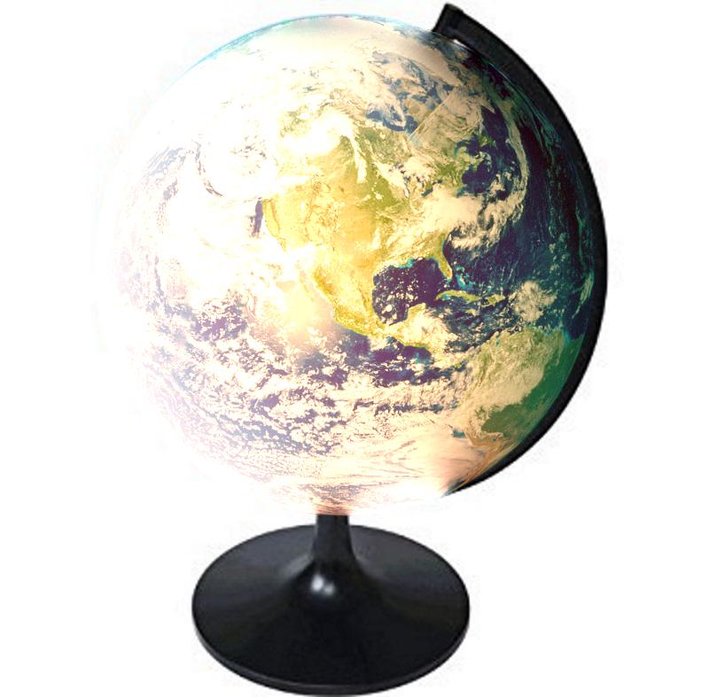
Part 2: Gradient Domain Fusion

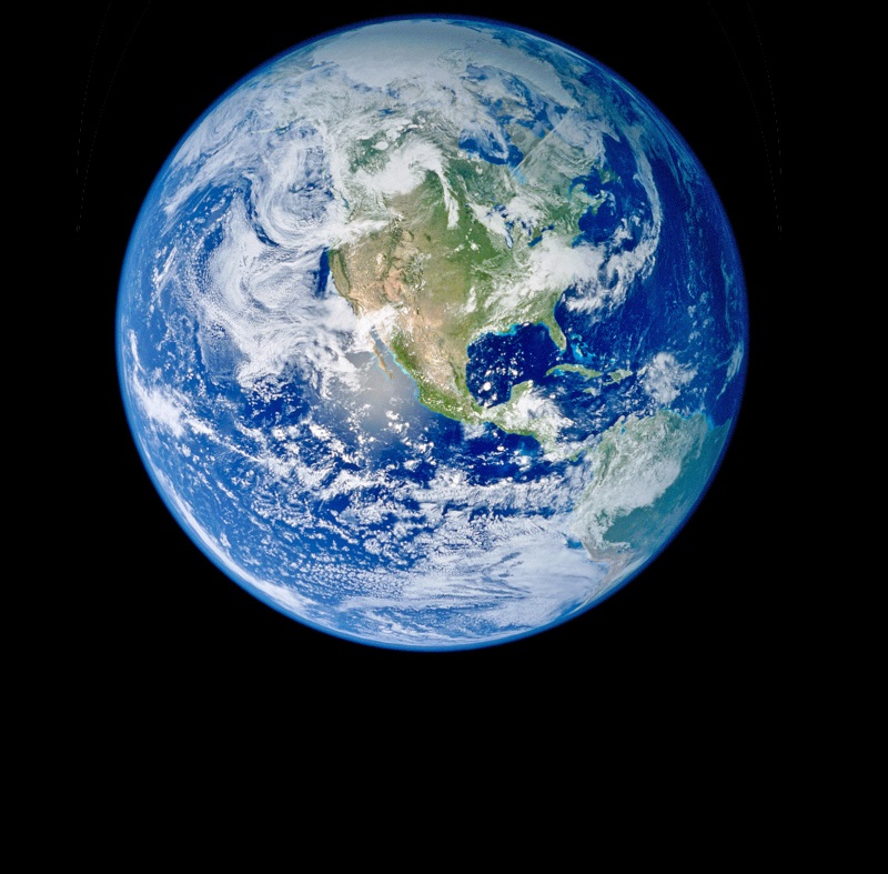
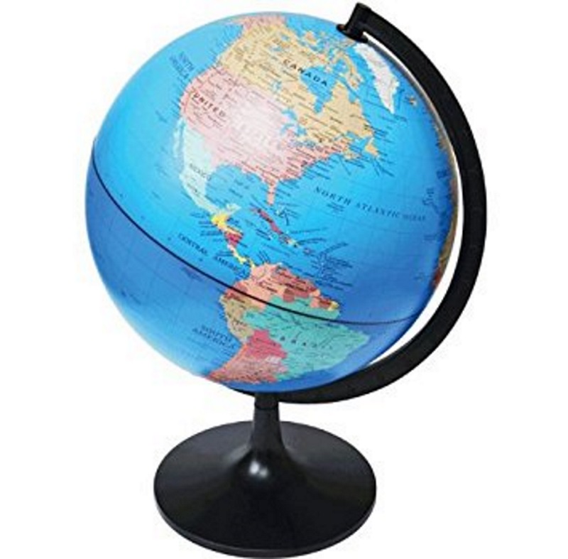
Multiresolution blending works well, however, it doesn't always do a good job on blending away seams. With starkly contrasted backgrounds (as in the globe example), portions can bleed over due to the Gaussian. Additionally, creating the masks can be time intensive as they need to be exact. This is where Poisson blending comes in. Given two images and an approximate mask, it can copy the source image to a different background seamlessly and without needing the user to create intricate masks.

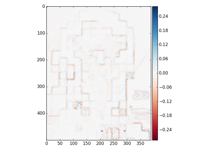
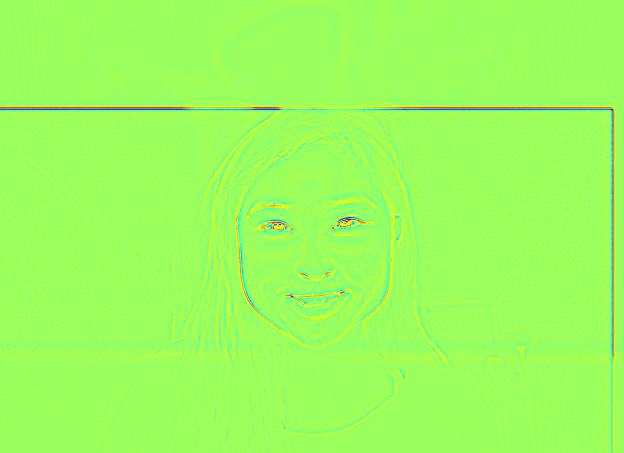
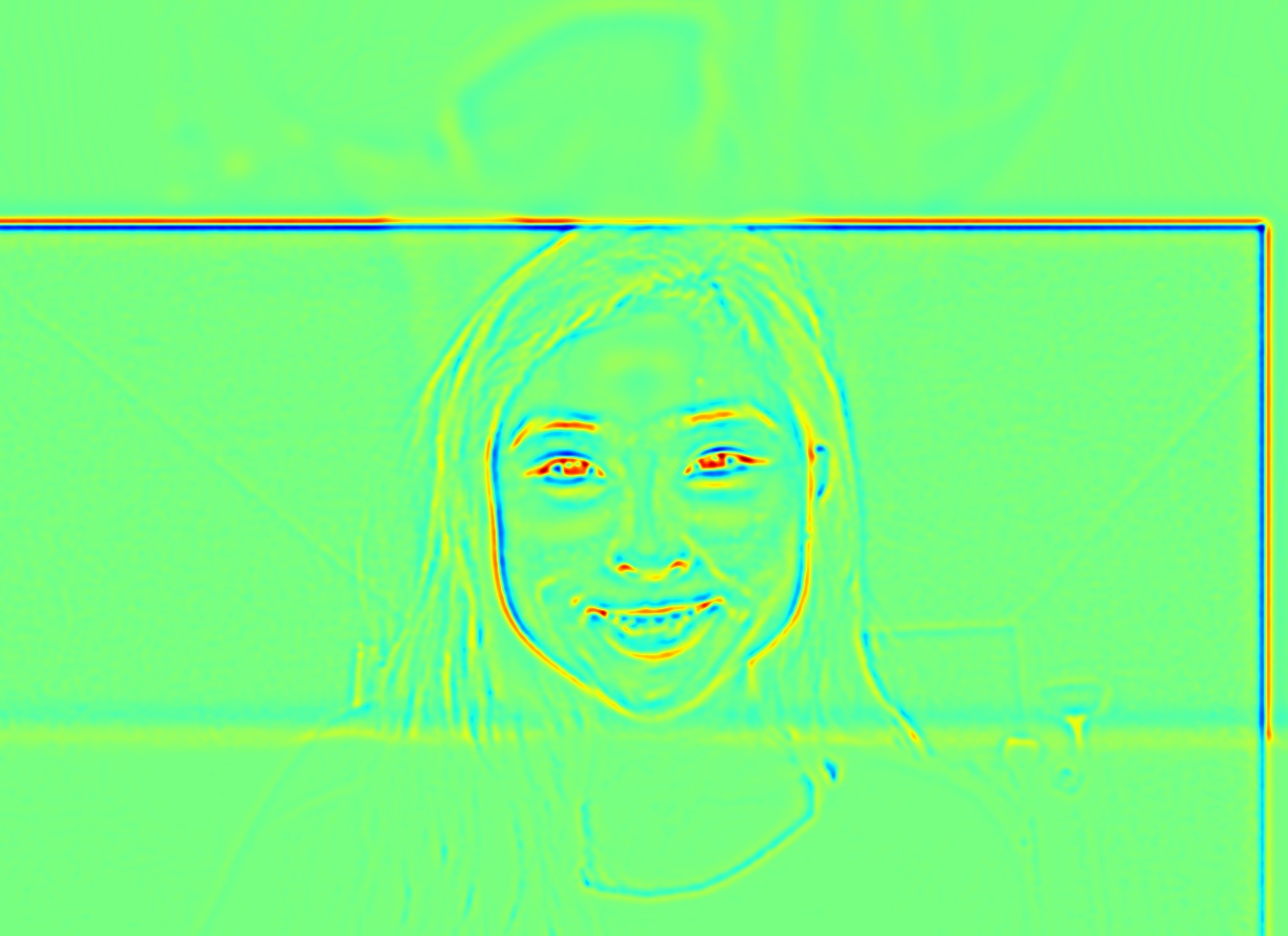
2.1: Toy Problem

In this section, I calculated the x-gradient and y-gradient of the input image to reconstruct the input image. The x-gradient is calculated by subtracting the source pixel from the neighboring pixel to the right for all pixels in the image (getting the x-gradinets). The y-gradient is calculated by subtracting the source pixel from the pixel above for all pixels in the image (getting the y-gradients)

I reconstructed Buzz and Woody as shown in the spec. The images aren't particularly impressive as I take in the input image, calculate the gradients to get a matrix of form Av = b where b contains the known values and A has the coefficients of the values we're looking for (which will be equivalent to b).

2.2: Poisson Blending

Favorite Example

Compare and Contrast: Multiresolution vs Poisson

Poisson blending is obviously better in this case as no extra work was necessary to colorize the image. Additionally, the multi-resolution blend sometimes bleeds onto the target background which is problematic. Poisson blending alters the colors of the source image though (as a key characteristic on how the method works) so if color constancy is important, then multiresolution with color will probably work better.