Introduction
In this project, I will be exploring different kinds of image blending and varies techniques. We will take advantage of passing different frequencies of an different images and blend them. Also we will explore blending images with respect to gradients.
Frequency Domain Blending
1.1 Image Sharpening using Unsharp Masking
1.1.1 Theorey
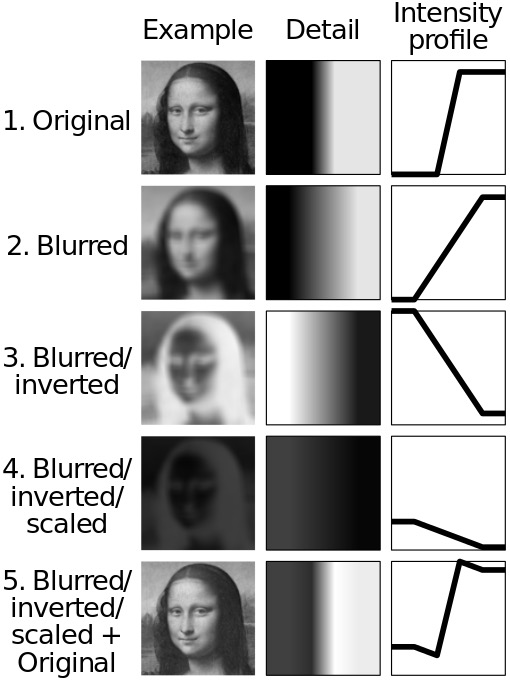
The 'unsharp' of the name derives from the fact that the technique uses a blurred, or 'unsharp', negative image to create a mask of the original image. The unsharped mask is then combined with the positive (original) image, creating an image that is less blurry than the original. Effectively, the resulting image will be sharpened.
sharpened image = f + α(f − f*g) = (1+α)f − αf*g = f * ( (1+α)e − αg ); where
    f is the original image
    α is the sharpening factor
    g is the gaussian kernel
    e is a dirac delta in 2d space sized same as gaussian kernel
 |
Step-by-step demostration1 |
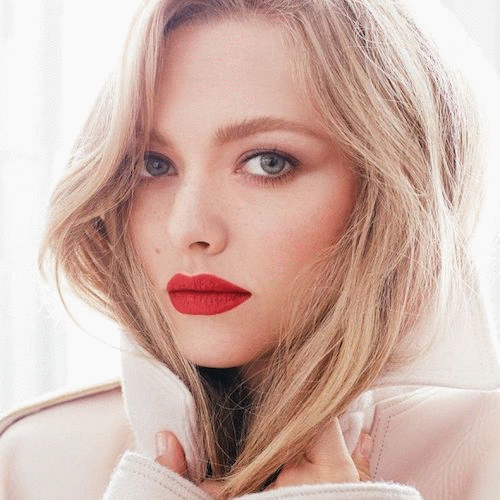
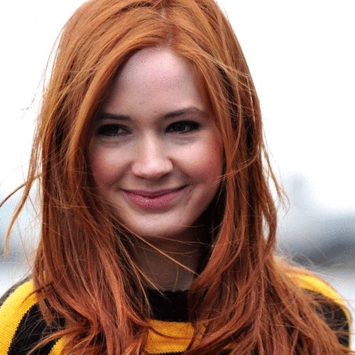
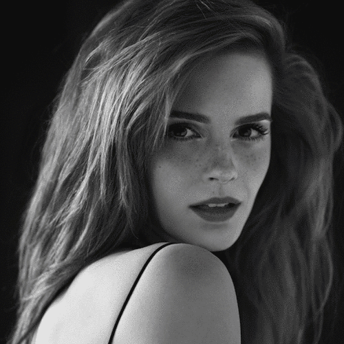
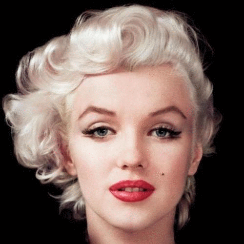
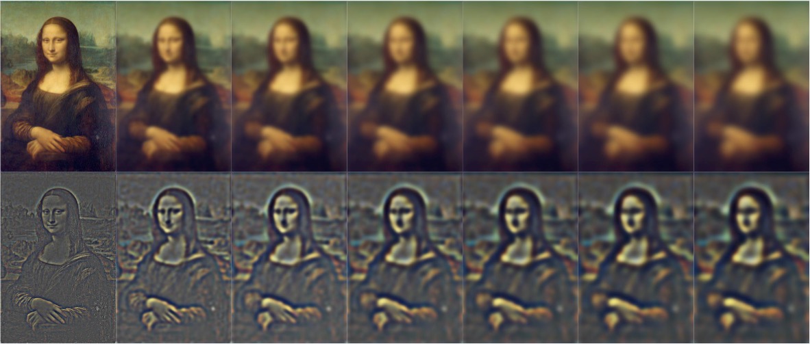
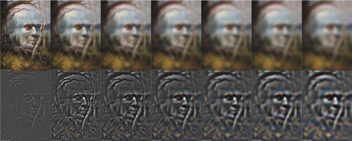
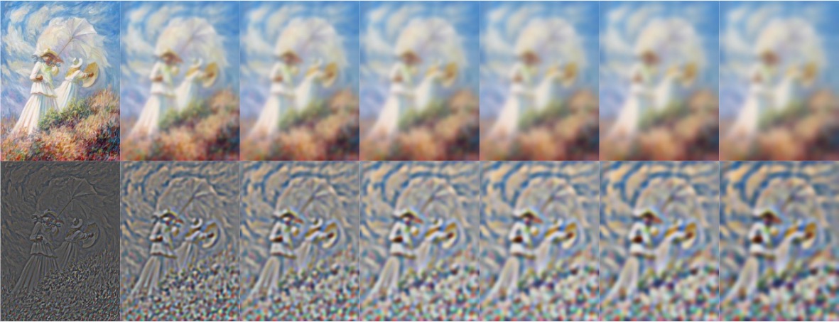
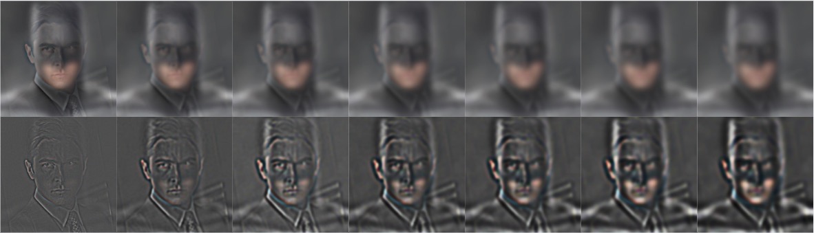
1.1.2 Results
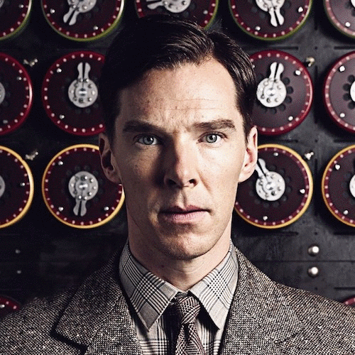
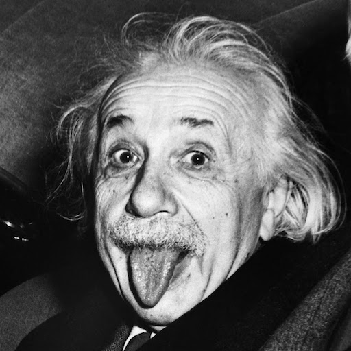
The results are gif animated. I chose a rather small sharpening factor α for a more natural result. You might need to zoom in the browswer to see the subtle difference. If you still can't see it, look into their eyes.
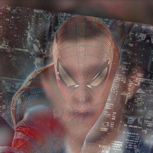
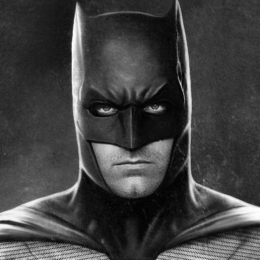
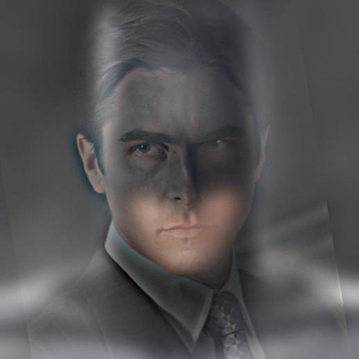
1.2 Hybrid Images
1.2.1 Theory
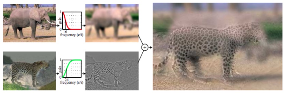
The goal of this part of the assignment is to create hybrid images using the approach described in the SIGGRAPH 2006 paper2 by Oliva, Torralba, and Schyns. Hybrid images are static images that change in interpretation as a function of the viewing distance. The basic idea is that high frequency tends to dominate perception when it is available, but, at a distance, only the low frequency (smooth) part of the signal can be seen. By blending the high frequency portion of one image with the low-frequency portion of another, you get a hybrid image that leads to different interpretations at different distances.
Lowpass image = f * g;
Highpass image = f - (f * g); where
    f is the original image
    g is the gaussian kernel
 |
Step-by-step demostration2 |
1.2.2 Results
Try to walk back and forth from a distance
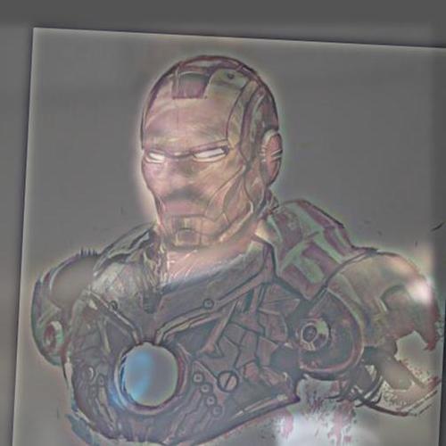
Not so successful results
 |
 |
 |
| Bigger on the Inside |
Fox |
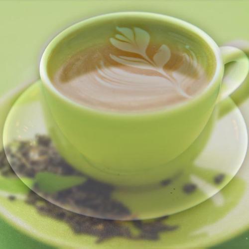
Tea or Coffee |
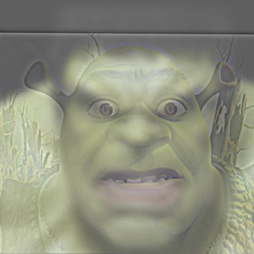
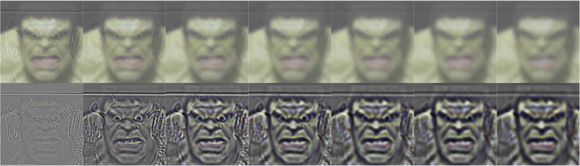
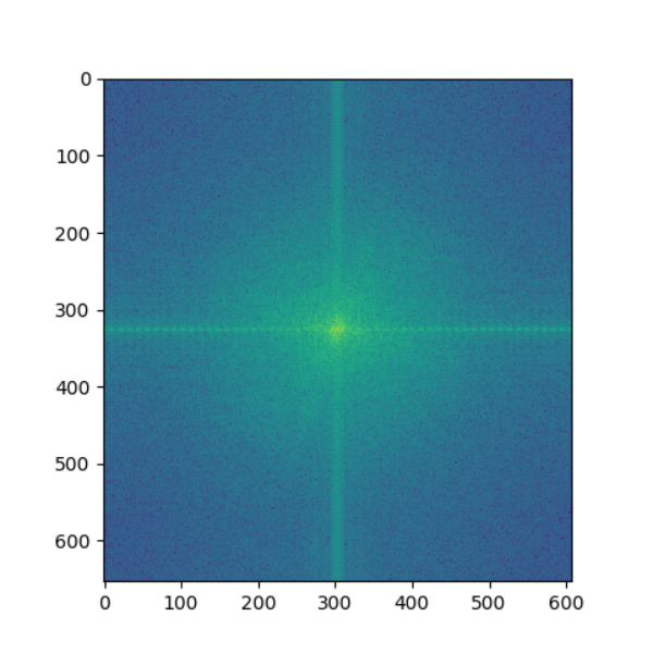
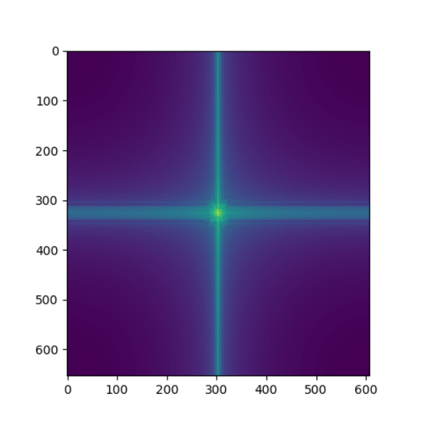
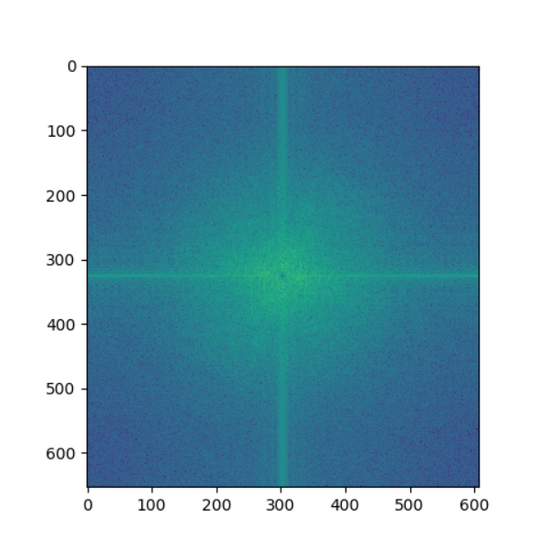
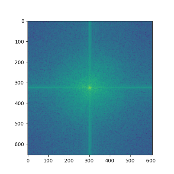
Frequency Domain Analysis on Hulk
 |
 |
 |
 |
 |
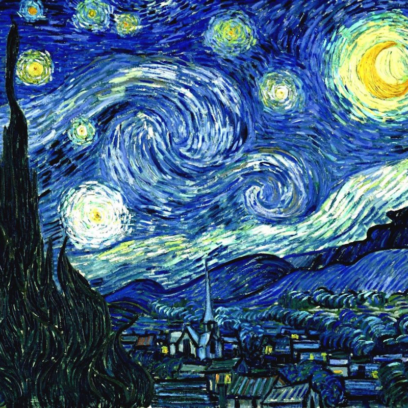
| Hulk original |
Shrek original |
Hulk low pass |
Shrek high pass |
Hybird image |
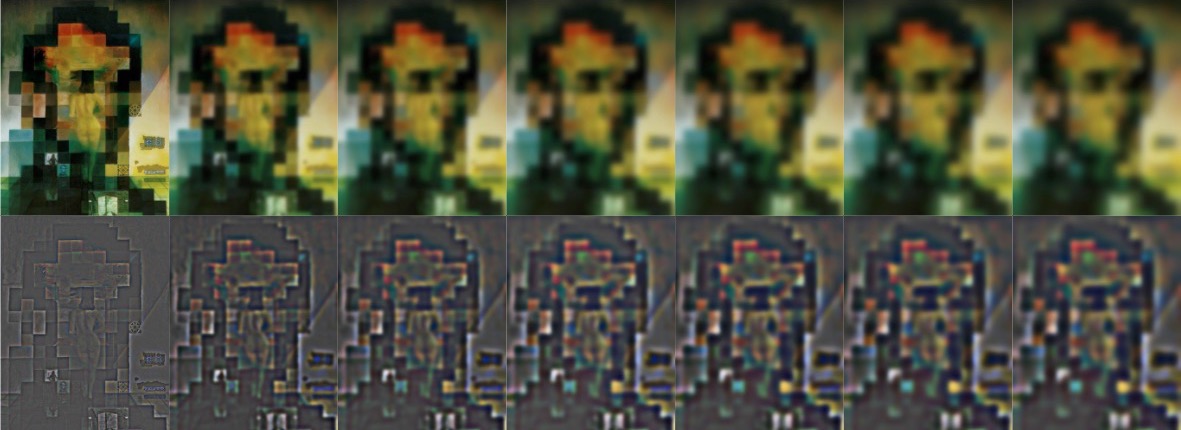
1.3 Hybrid Images
1.3.1 Theory
In this part I will implement Gaussian and Laplacian stacks. As a result, we can analyse images in different frequency bands.
Li = Gi - Gi+1; where
    Li is the ith Laplacian image
    Gi is the resulting image from applying gaussian blur i times.
1.3.2 Results
Gaussian and Laplacian decomposition of complex images
1.4 Multiresolution Blending
1.4.1 Theory
The goal of this part is to blend two images seamlessly using a multi resolution blending as described in the 1983 paper3 by Burt and Adelson. An image spline is a smooth seam joining two image together by gently distorting them. Multiresolution blending computes a gentle seam between the two images seperately at each band of image frequencies, resulting in a much smoother seam.
BlendedImage = sum([LSk(i,j)]) + GA-1(i,j) + GB-1(i,j)  //Sum of all masked Laplacian of images A and B and the final masked Gaussian of image A and B.
LSk(i,j) = GMk(i,j) * LAk(i,j) + (1 - GMk(i,j) * LBk(i,j)); where
    GXk(i,j) is the kth Gaussian image X
    LXk(i,j) is the kth Laplacian image of the image X
    A is image A
    B is image B
    M is the mask
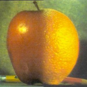
1.4.2 Results + Bells and Whistles (Colour images)
Results of multiresolution belaning
 |
 |
 |
 |
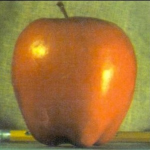
| Apple |
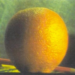
Orange Man |
Mask |
Orapple |
 |
 |
 |
 |
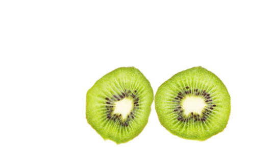
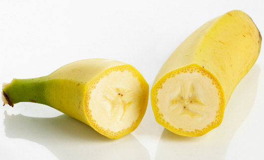
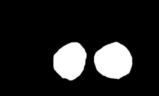
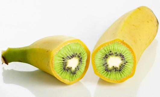
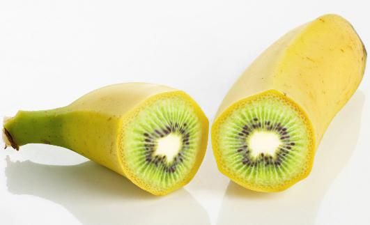
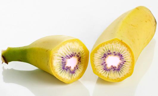
| Kiwi |
Banana Man |
Mask |
Kiwana |
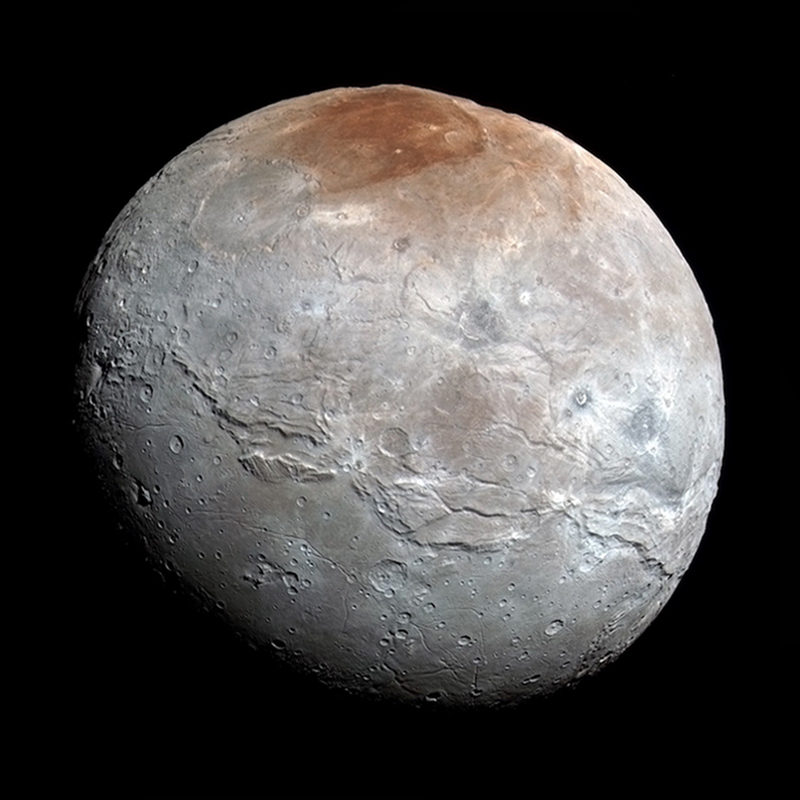
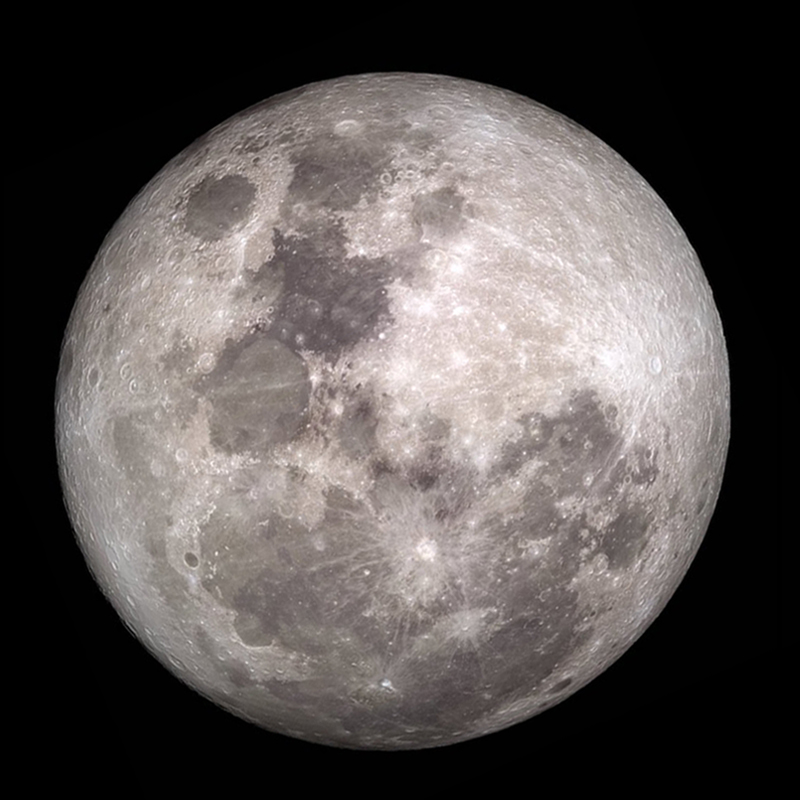
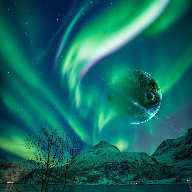
Analysis and decomposition on Pluoon (Gif animated)
Gradient Domain Blending
2.1 Toy Problem
2.1.1 Theory
The goal of this part is to reconstruct a whole image from only gradient data and a signle pixel as a constrain.
minimise (vi[x+1,y]-vi[x,y] - (si[x+1,y]-si[x,y]))2
minimise (vi[x,y+1]-vi[x,y] - (si[x,y+1]-si[x,y]))2
minimise (v[0,0]-s[0,0])2 ; where
    xi is the ith pixel of the flattened image x
    v is the resulting image
    s is the source image
2.1.2 Result
The image in the right has been reconstructed from extrating the gradient from the left image and a single pixel at [0,0].
 |
 |
| Original |
Reconstructed |
2.2 Poisson Blending
2.2.2 Theory
The primary goal of this assignment is to seamlessly blend an object or texture from a source image into a target image. The simplest method would be to just copy and paste the pixels from one image directly into the other. Unfortunately, this will create very noticeable seams, even if the backgrounds are well-matched. How can we get rid of these seams without doing too much perceptual damage to the source region?
One way to approach this is to use the Laplacian pyramid blending technique we implemented for the last project. Here we take a different approach. The insight we will use is that people often care much more about the gradient of an image than the overall intensity. So we can set up the problem as finding values for the target pixels that maximally preserve the gradient of the source region without changing any of the background pixels. Note that we are making a deliberate decision here to ignore the overall intensity! So a green hat could turn red, but it will still look like a hat.
We can formulate our objective as a least squares problem. Given the pixel intensities of the source image "s" and of the target image "t", we want to solve for new intensity values "v" within the source region "S"
Here, each "i" is a pixel in the source region "S", and each "j" is a 4-neighbour of "i". Each summation guides the gradient values to match those of the source region. In the first summation, the gradient is over two variable pixels; in the second, one pixel is variable and one is in the fixed target region.
The method presented above is called "Poisson blending". Check out the Perez et al. 2003 paper3 to see sample results. This is just one example of a more general set of gradient-domain processing techniques. The general idea is to create an image by solving for specified pixel intensities and gradients.
v = argminv = ΣiϵS,jϵNi∩S ((vi-vj)+(si-sj))2 + ΣiϵS,jϵNi∩¬S ((vi-tj)+(si-sj))2; where
    vi is the ith pixel of the resulting image
    S is the set of pixels in source image
    jϵNi∩S are the neighbours of pixel i whilst the neighbours are in the mask
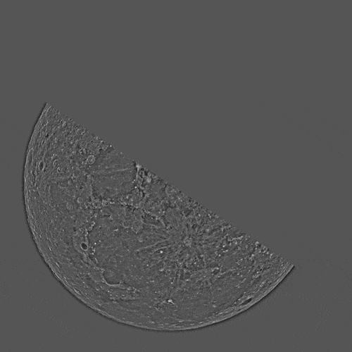
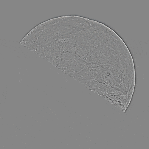
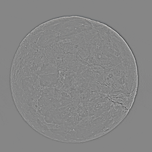
2.2.2 Result
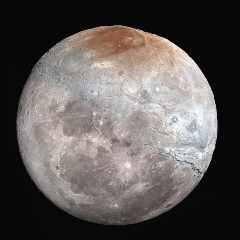
The image has been blended from Moon and Pluto. The result from Poisson Blend is stunning. One thing is that we have to make sure the two planets are aligned well beofre blending.
 |
| Poisson Blend |
 |
 |
 |
| Source |
Target |
Naive Blend |
2.2.2 More Results
More Poisson Blending Results shown.
 |
 |
 |
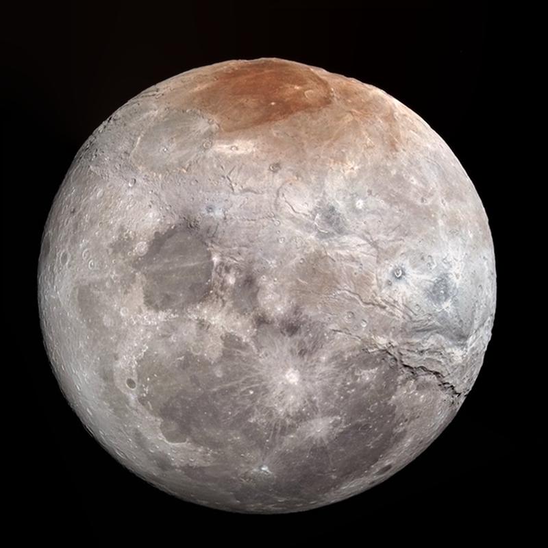
| New Moon |
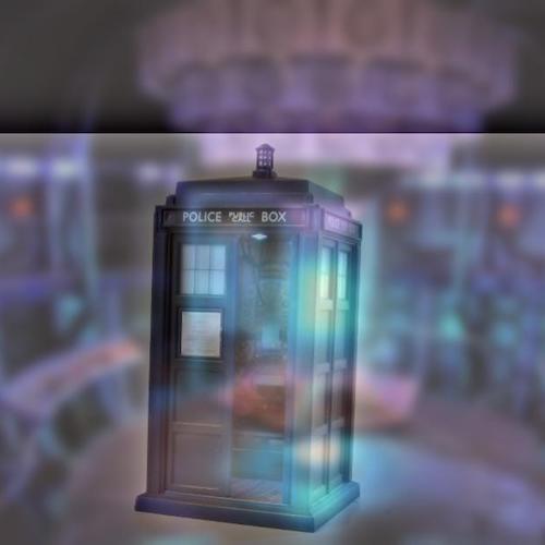
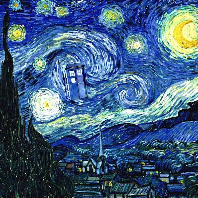
Tardis |
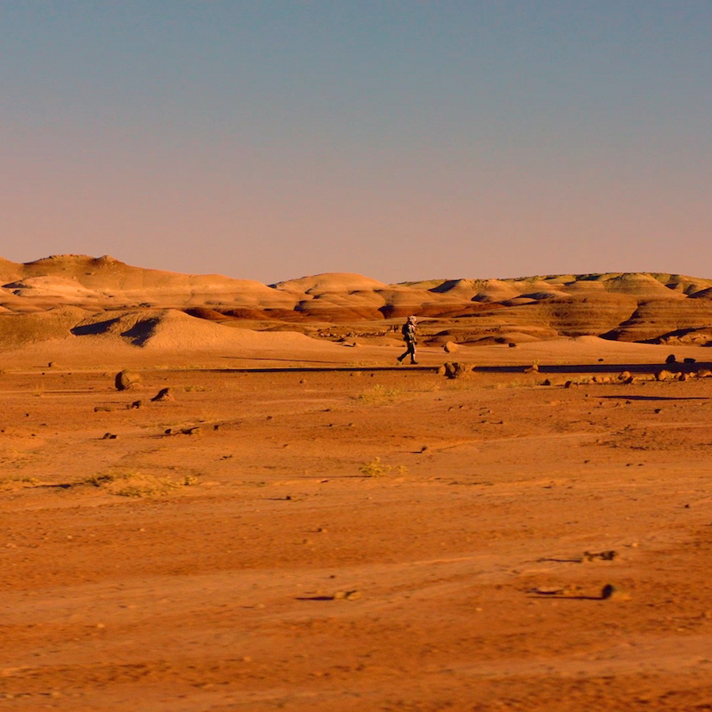
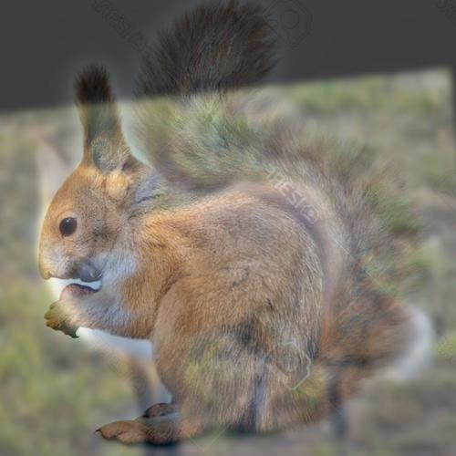
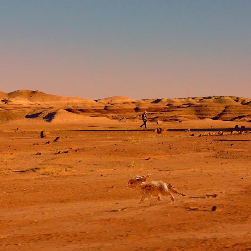
Fox on Mars |
2.2.3 Comparism between Naive Blend, Laplacian Blend and Possion Blend
We can see Laplacian Blend does pretty when when edge of source is close in colour to target. We also see that since Possion Blend minimises the edge differemce, it sacrifices the hue of the source image despite the correct gradient.
 |
 |
 |
| Naive Blend |
Laplacian Blend |
Possion Blend |
1https://en.wikipedia.org/wiki/Unsharp_masking
2http://cvcl.mit.edu/publications/OlivaTorralb_Hybrid_Siggraph06.pdf
3http://persci.mit.edu/pub_pdfs/spline83.pdf
3http://cs.brown.edu/courses/csci1950-g/asgn/proj2/resources/PoissonImageEditing.pdf