Part 1.1: Warmup
To sharpen the image I simply applied a laplacian filter and added the result back to the original.
| original | sharpened |
 |
 |
To sharpen the image I simply applied a laplacian filter and added the result back to the original.
| original | sharpened |
| |
|
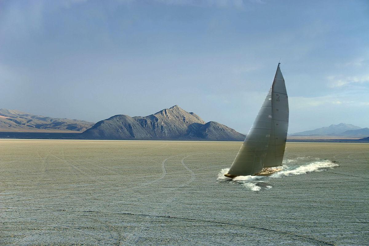
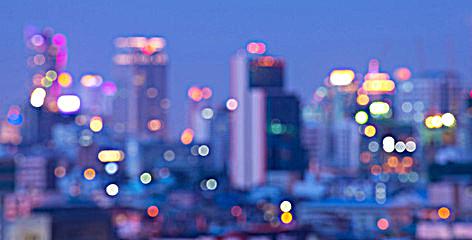
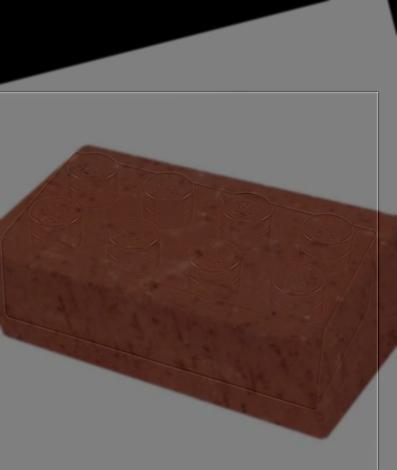
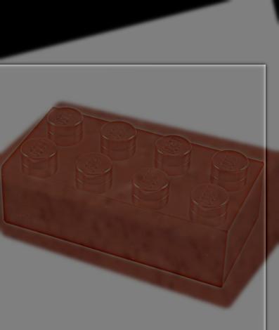
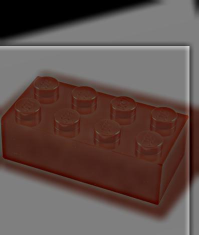
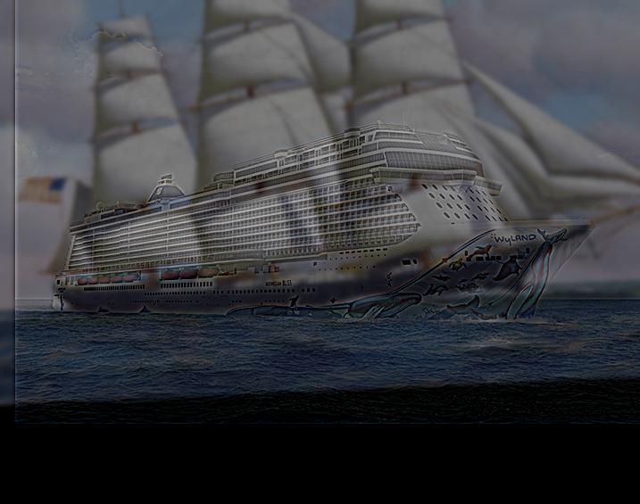
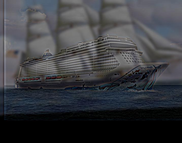
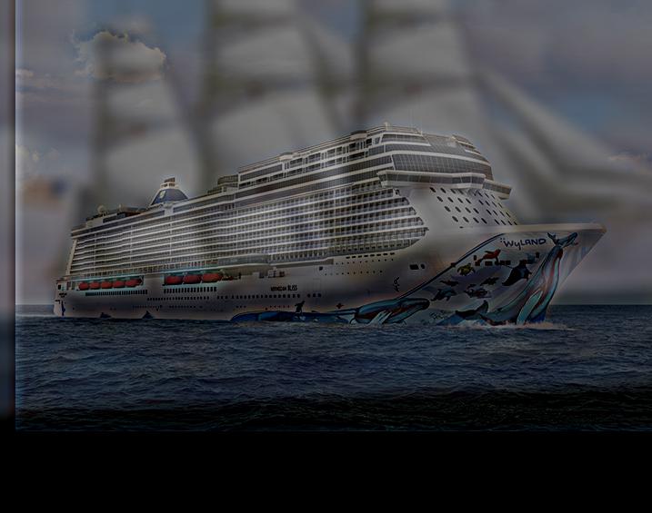
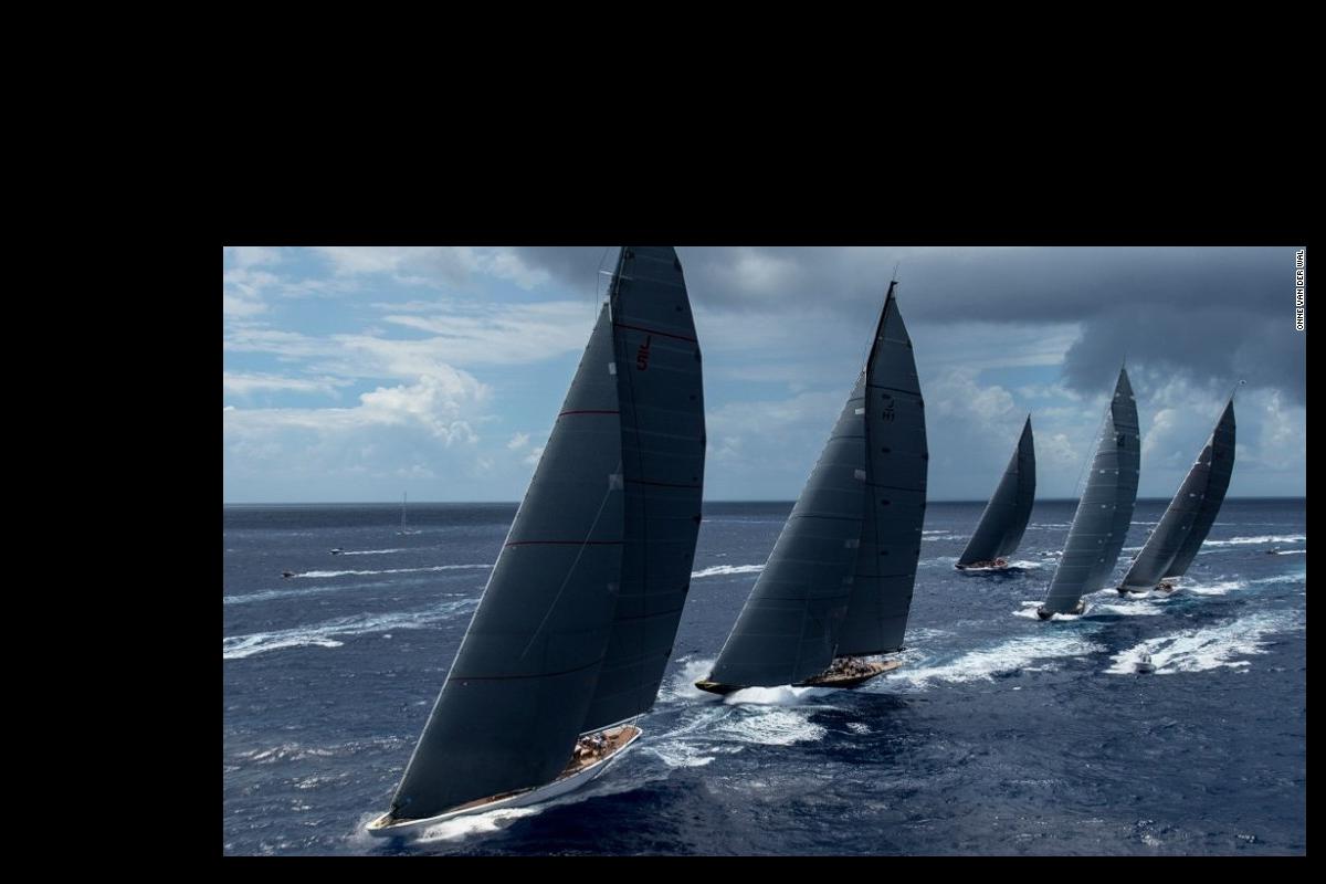
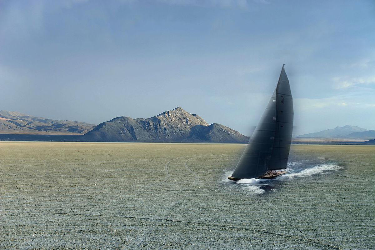
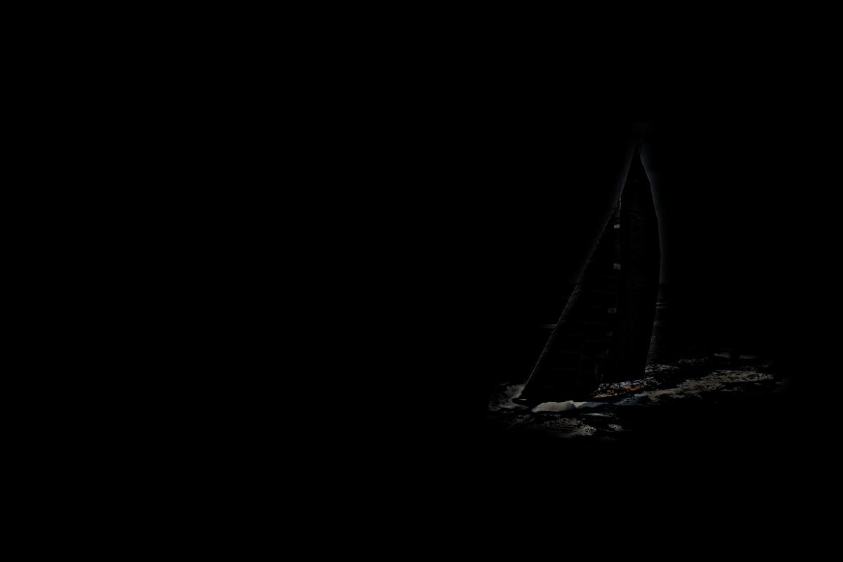
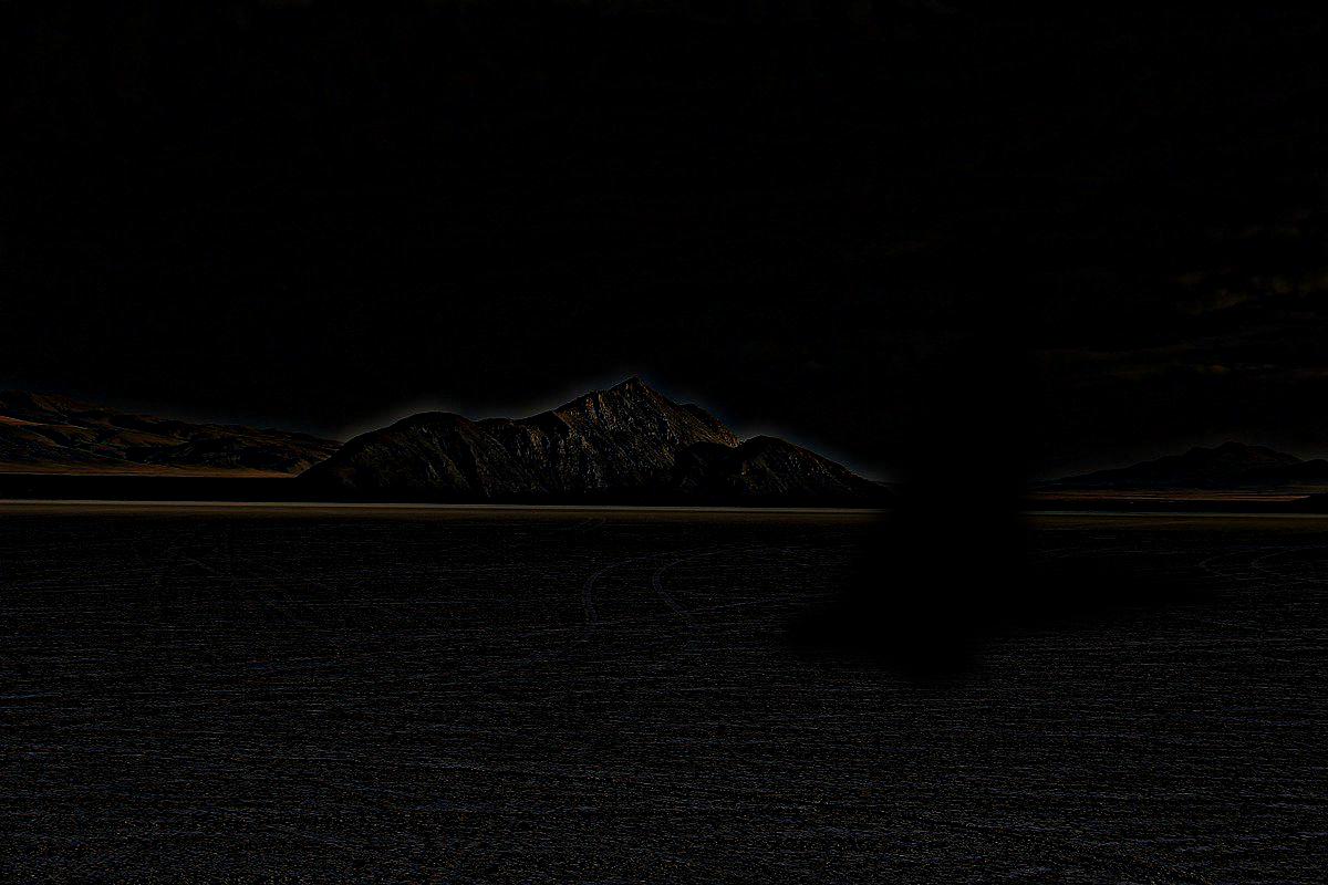
To find the best cut-off frequency for the images I simply tried several different filters for each hybrid image. The standard deviations for the gaussian kernels that I experimented with were 1, 2.5, 5, and 10. I chose these pairing based on their similar shapes as well as their similar colors.
| sigma=1 | sigma=2.5 | sigma=5 | sigma=10 |
 |
 |
 |
 |
 |
 |
 |
 |
| |
|
| original Lego brick image | original brick image | gaussian filtered Lego brick image | laplacian filtered brick image | hybrid image |
 |
 |
 |
 |
 |
For the laplacian and gaussian stacks I used a standard deviation of 7 and 5 for the kernels respectively.
 |
 |
 |
 |
 |
 |
 |
 |
 |
 |
 |
 |
 |
 |
 |
 |
 |
 |
 |
 |
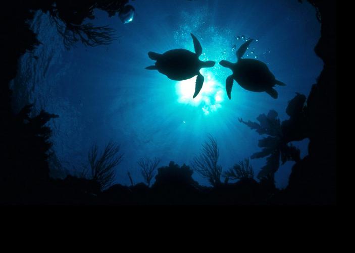
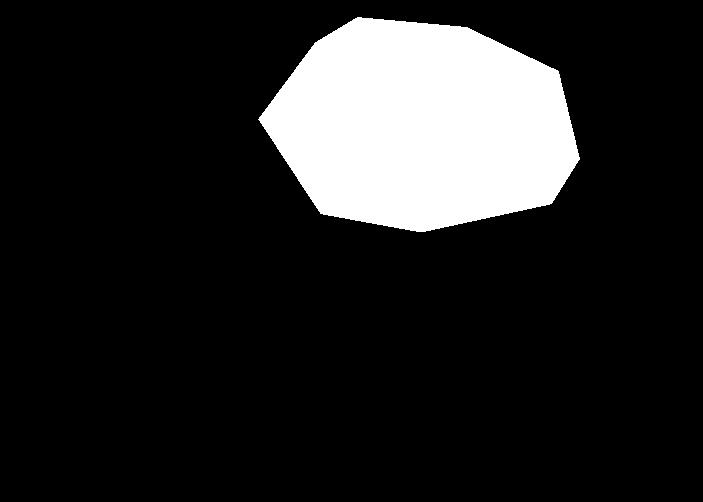
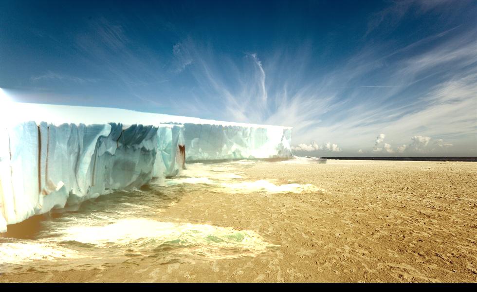
To contruct the A and b matrices I used a very similar method to the Toy Problem. I constructed the coefficient matrix such that each row contained the weights of the laplacian matrix and the b matrix was the result of convolving the composed target-source image with the same laplacian matrix.

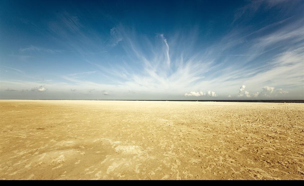
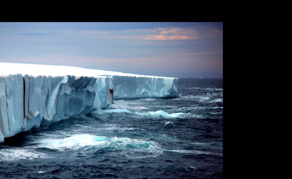
| target | source | mask |
 |
 |
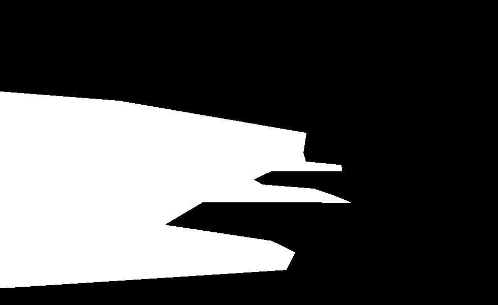 |
| target | source | mask |
 |
 |
 |
| target | source | mask |
 |
 |
 |
| target | source | mask |
| |
|
|
 |
 |
 |
 |
 |
 |
 |
 |
 |
 |
 |
 |
 |
 |
 |
 |
 |
 |
To contruct the coefficient matrix for the least squares solver, I created two rows for each pixel of the image in addition to one row to contrain the value of the first pixel. Each row has mxn columns, with each column representing the coefficient corresponding to that pixel. In the end, all but the last row has exactly one entry equal to 1 and another equal to -1. These coefficients come from the 1 and -1 coefficients of the contraints min( v(x,y+1)-v(x,y) - (s(x,y+1)-s(x,y)) )^2 and min( v(x+1,y)-v(x,y) - (s(x+1,y)-s(x,y)) )^2. The last row has a 1 in the first column. The b vector of the least squares solver is equaled to the flattened imaged that has been convolved with a [-1, 1] and [-1, 1]^T matrix. The last entry of the b vector is equal to the top right pixel of the original image.
| original | solution |
 |
 |
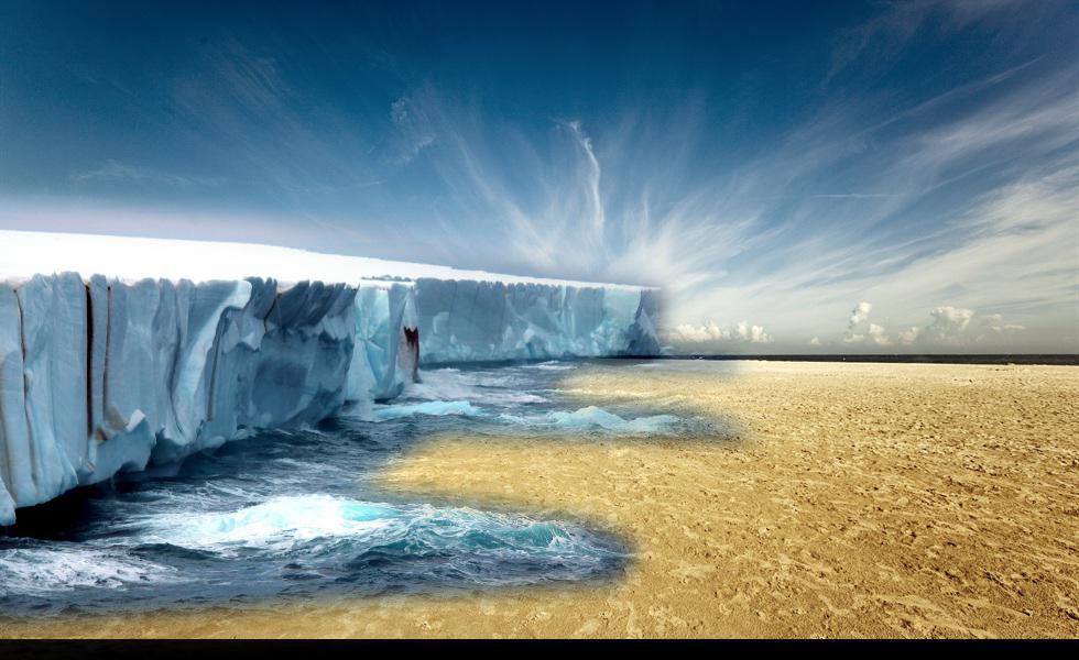
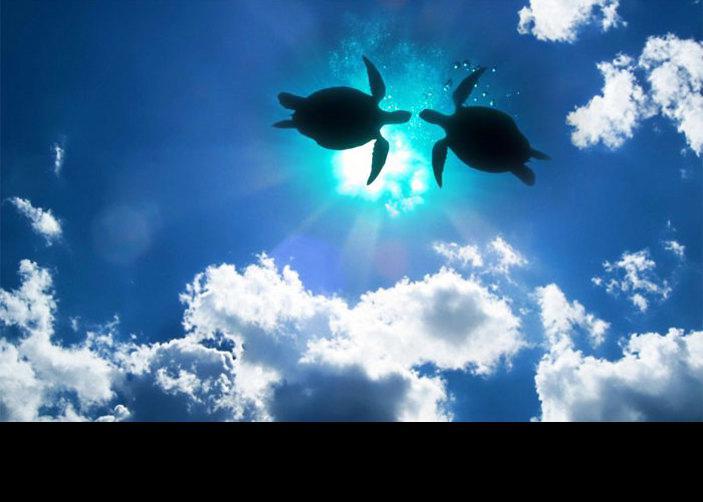
To contruct the A and b matrices I used a very similar method to the Toy Problem. I constructed the coefficient matrix such that each row contained the weights of the laplacian matrix and the b matrix was the result of convolving the composed target-source image with the same laplacian matrix. Overall, I think these images turned out much better than the multiresolution blended pictures, because the mask is less visible and the color of the source image adjusts to the surrounding colors of the target image.
| target | source | mask |
| |
|
|
| target | source | mask |
| |
|
|
| target | source | mask |
| |
|
|