CS194-26 Project 3
Part 1.1 - Sharpening an image
For this part, I used the unsharp mask filter that was taught in class. The procedure was the following:
- Blur the image using a gaussian filter to get a low pass filtered image. In this case, I used a sigma of 5.
- Subtract the blurred version from the original image to get a high pass filter of the original, making sure to clip the image values from 0 to 1.
- Add the high pass filtered image back to the original with a weight alpha. I picked 0.9.

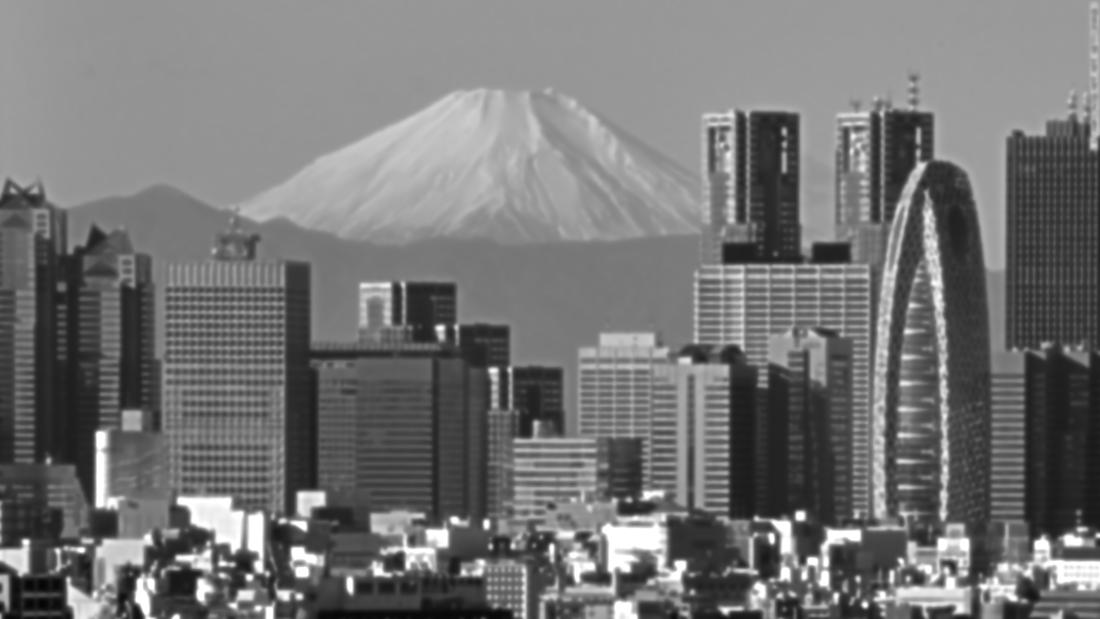
Original Image
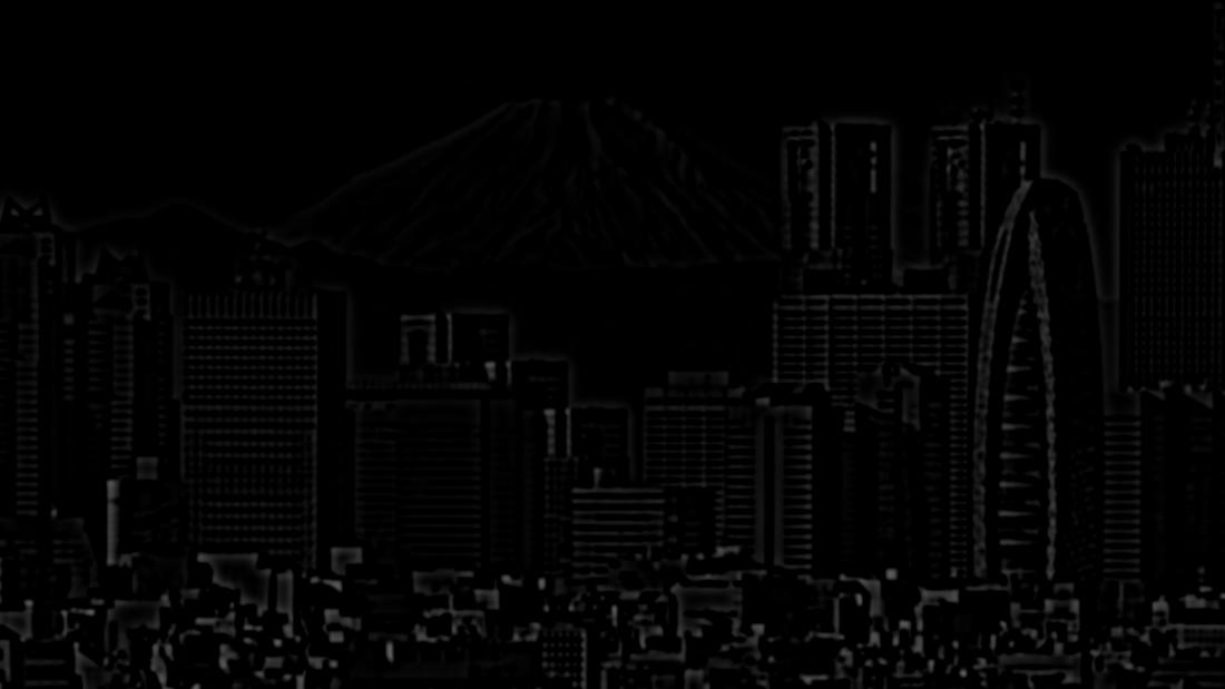
High Pass Filter
Sharpened Image
Part 1.2 - Hybrid Images
In this part, we create hybrid images using the following procedure:
- Use the starter code to get the points that align two images I and I'
- Apply a gaussian filter on I to get its low frequency components
- Apply a high pass filter on I' by computing the gaussian on I' and subtracting that from the original I'
- Average the result of the low pass and high pass filters
Favorite Result
Input Images:

Obama
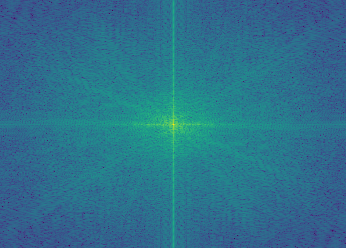
Original Obama Image FFT
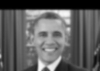
Obama Low Pass (sigma = 3)
Low Pass Obama Image FFT
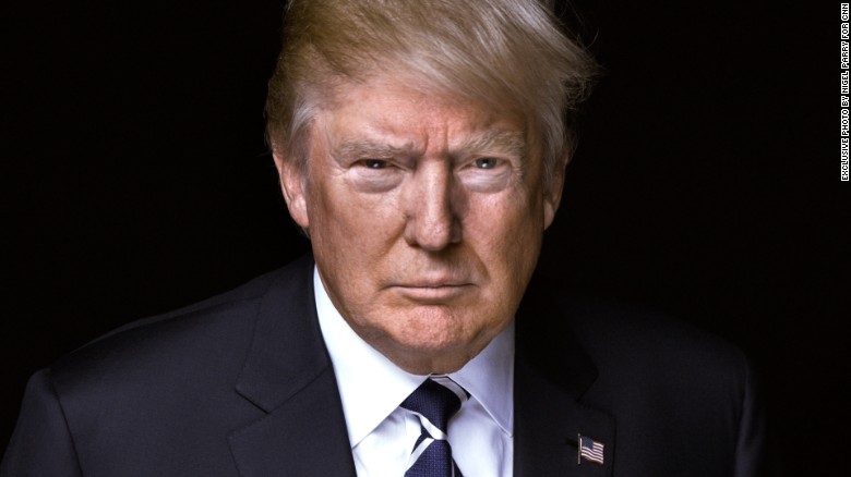
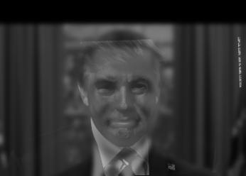
Trump
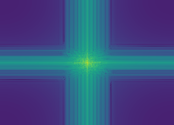
Original Trump Image FFT
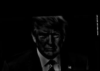
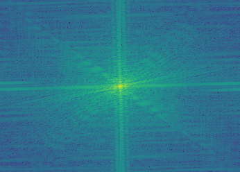
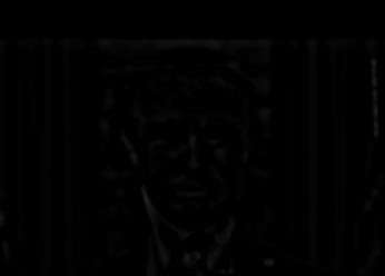
Trump High Pass (sigma = 10)

High Pass Trump Image FFT
Output Image:
Donald Obama

Donald Obama FFT
Other Results
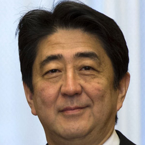
Shinzo Abe (Sigma = 6)

Kim Jong Un (Sigma = 4)
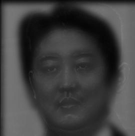
Abe Kim
Failure Case: Tiger Bulldog
I believe this case fails because the images are too dissimilar so the combined result at a distance does not look like the dog at all.
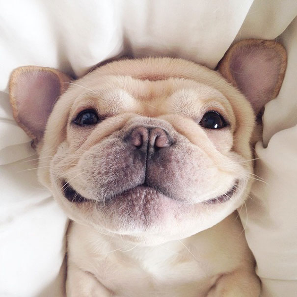
Bulldog (Sigma = 5)
Tiger (Sigma = 10)
Bulldog Tiger
Part 1.3 - Gaussian/Laplacian Stacks
To create the gaussian stack, I simply applied a gaussian filter with a sigma at increasing powers of two until 32.
For the Laplacian stack, I simply just took the difference between adjacent levels of the gaussian stack. The final level is just a normal gaussian though.
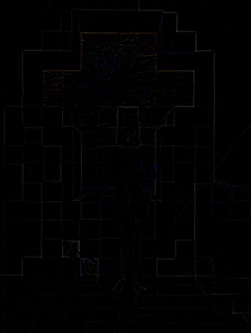
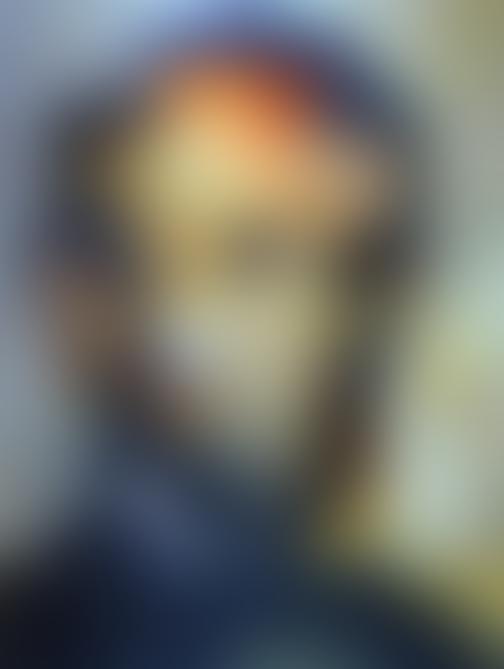
Dali's Lincoln Image Stacks
Gaussian Stack

Sigma = 0
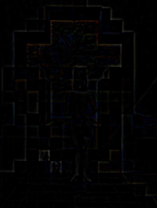
Sigma = 1

Sigma = 2

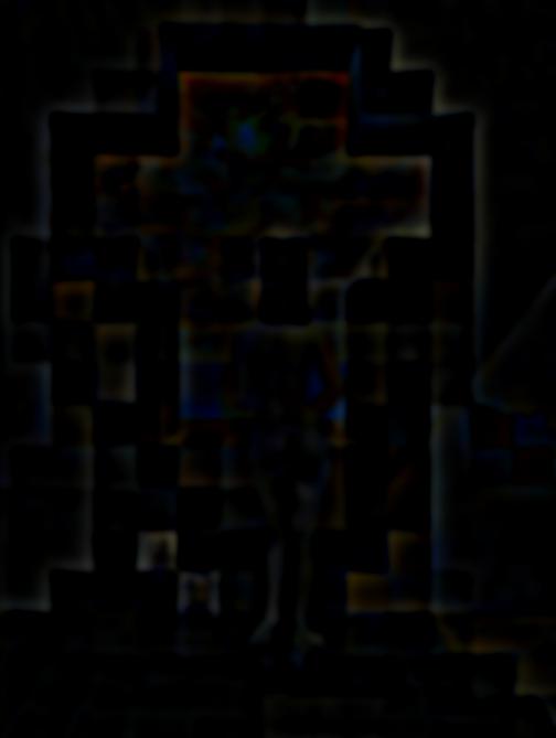
Sigma = 4

Sigma = 8

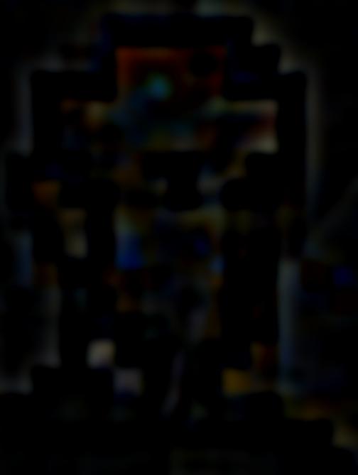
Sigma = 16

Sigma = 32
Laplacian Stack
g0-g1
g2-g1
g4-g2
g8-g4
g16-g8

g32-g16
g32
Donald Obama
Gaussian Stack

Sigma = 0

Sigma = 1

Sigma = 2

Sigma = 4

Sigma = 8
Sigma = 16

Sigma = 32
Laplacian Stack
g0-g1
g2-g1
g4-g2

g8-g4
g16-g8
g32-g16

g32
1.4 - Multiresolution Blending
We implement multiresolution to combine images with a less noticable seam via the following procedure:
- Create a gaussian stack of the mask, and Laplacian stacks for the two input images
- For each level in the three stacks, weigh one image's level in the laplacian by the gaussian of the mask at that level, and the other image's laplacian of that level by the complement of the gaussian of the mask
- Flatten all the levels into one image
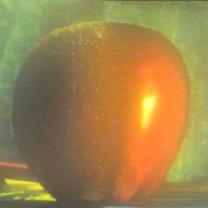
Oraple

Orange

Apple
Mask
Result
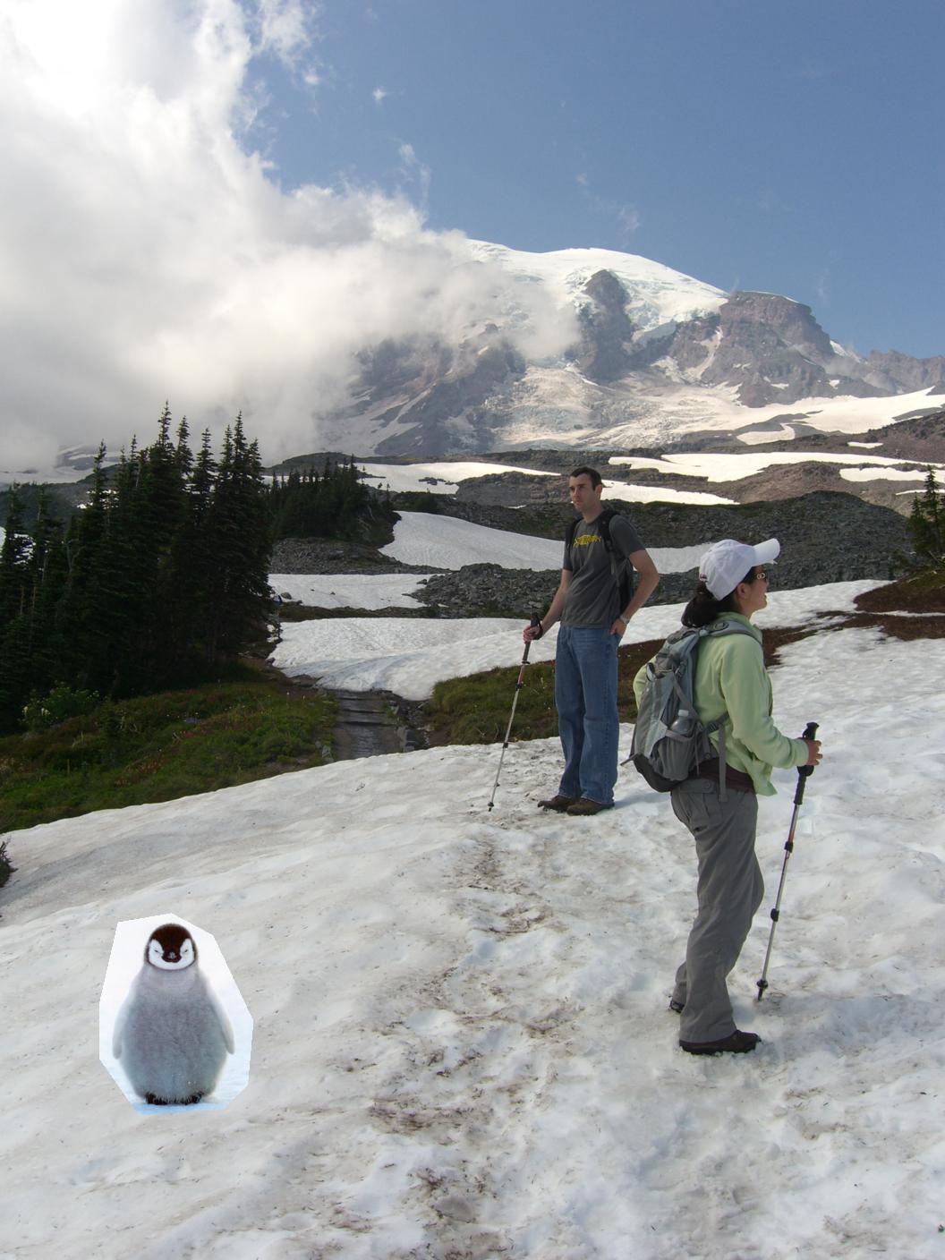
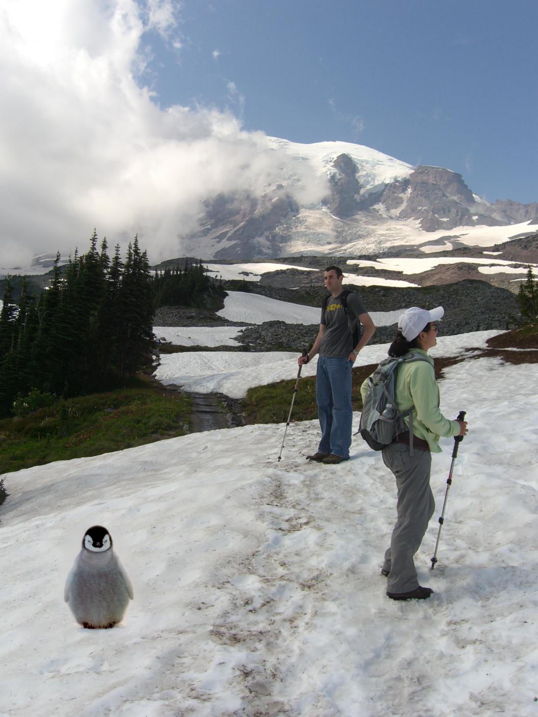
Irregular Mask: Penguin with Skiers
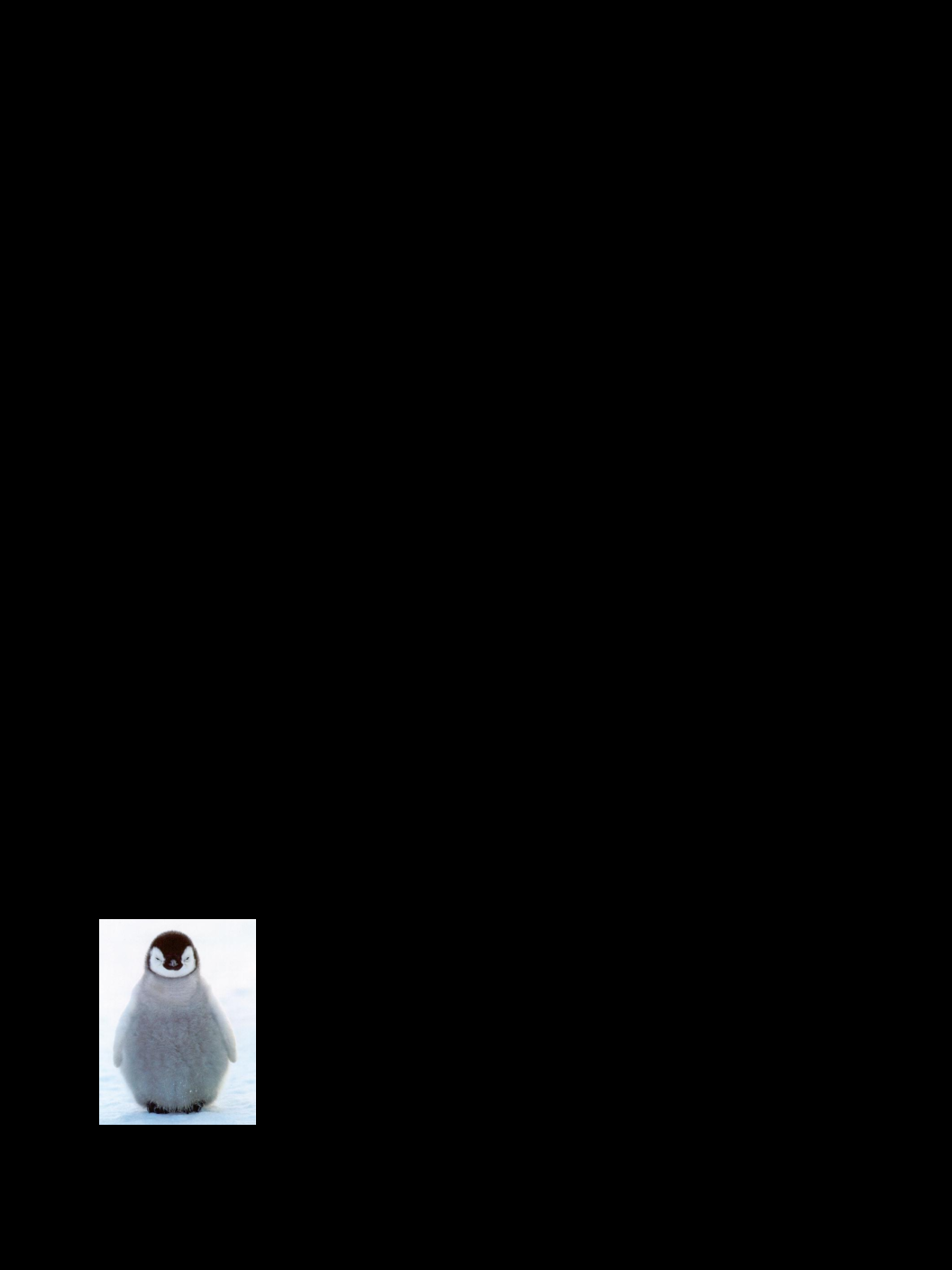
Penguin
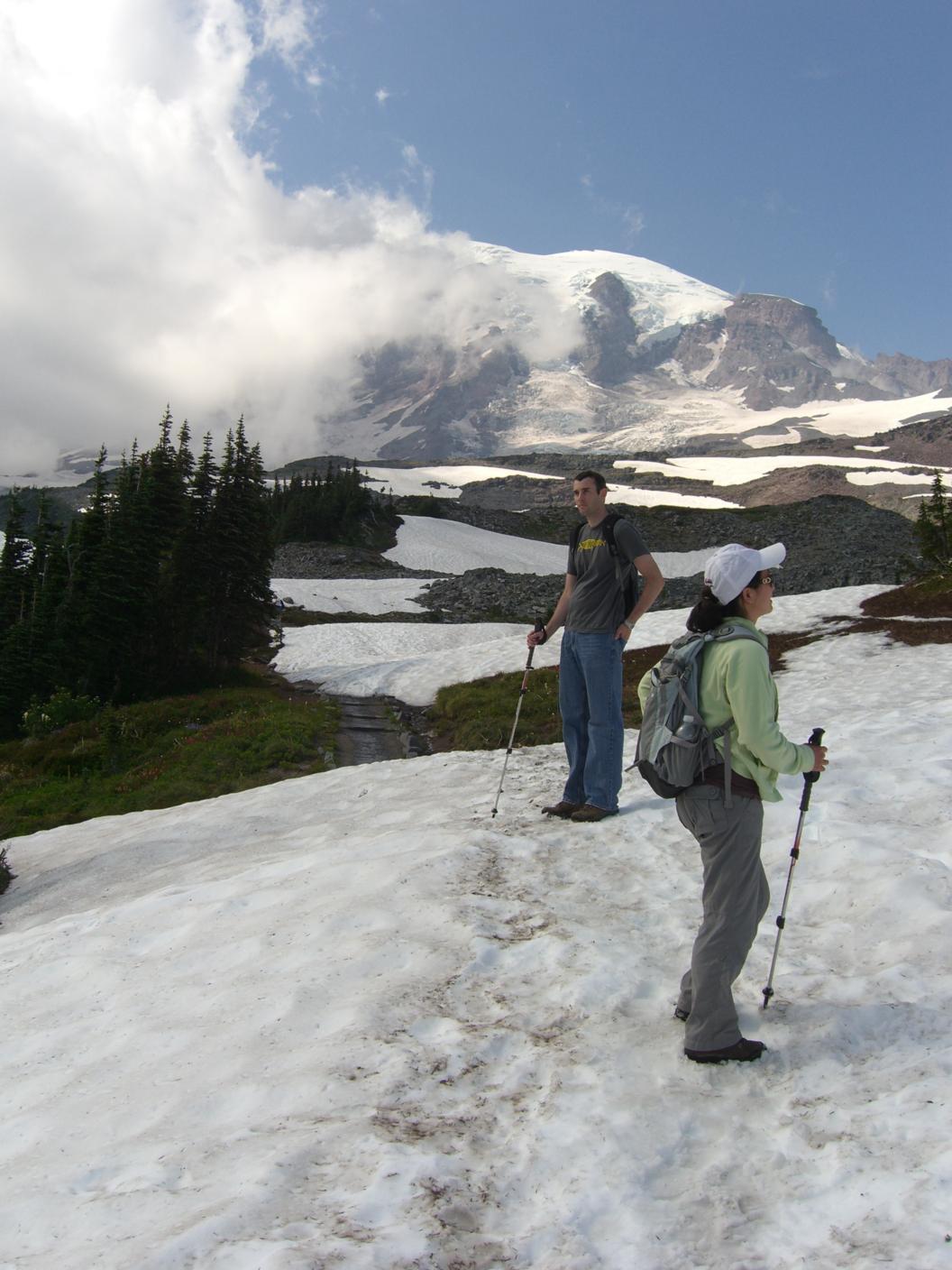
Skiers
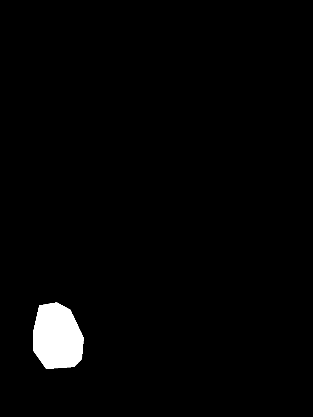
Mask
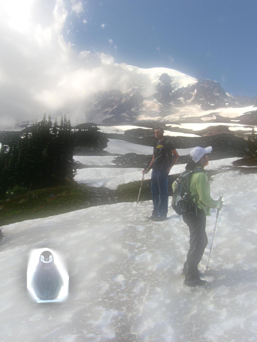
Penguin with Skiers
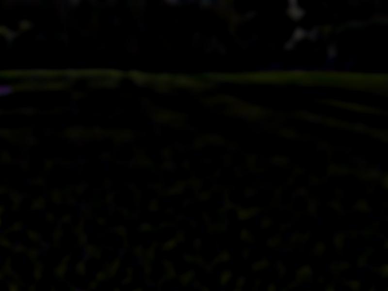
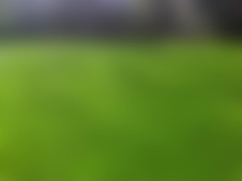
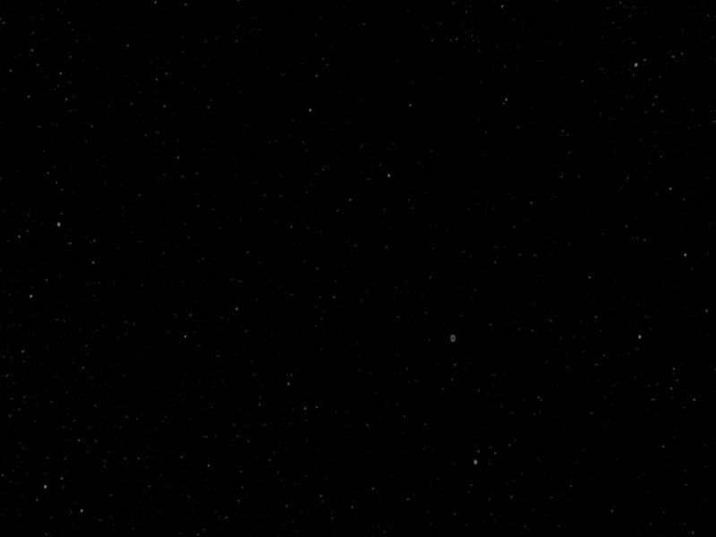
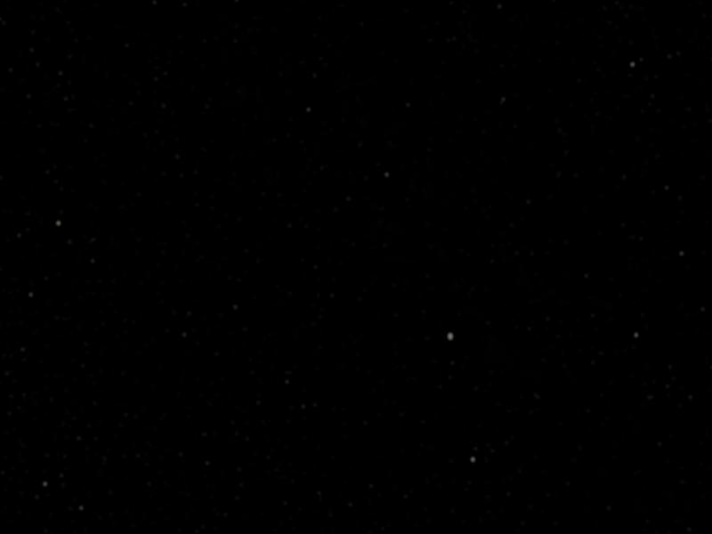
Favorite: Space Grass
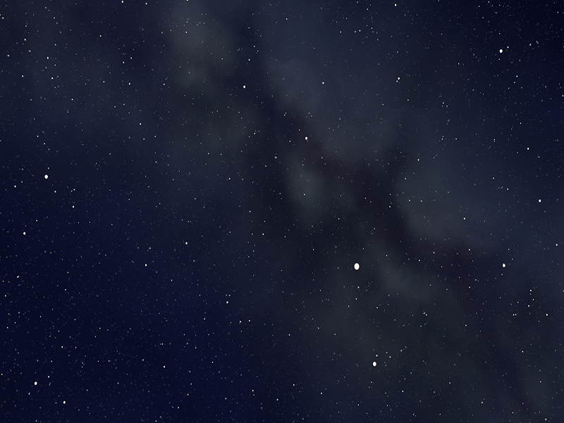
Space Dust
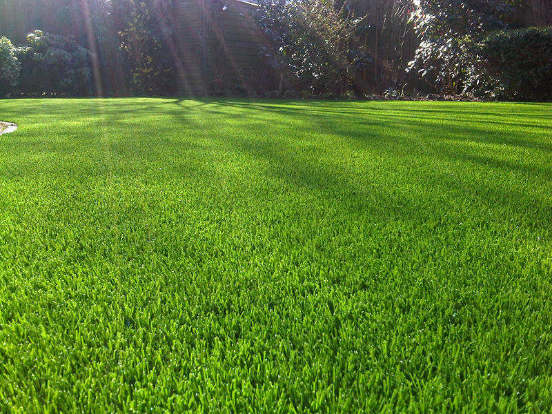
Grass

Mask
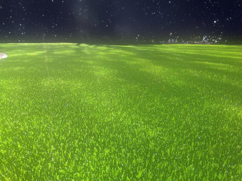
Result
Laplacian Stack of grass
g0-g1
g2-g1
g4-g2
g8-g4
g16-g8

g32-g16
g32
Laplacian Stack of space

g0-g1
g2-g1
g4-g2
g8-g4

g16-g8
g32-g16

g32
Gaussian Stack of mask

Sigma = 0

Sigma = 1

Sigma = 2

Sigma = 4

Sigma = 8

Sigma = 16

Sigma = 32
Bells and whistles
Note that color was used for these images!
Part 2
Overview
In this part, we investigate how to perform processing in the gradient domain in order to more seamlessly blend images together. The main idea behind this part is that instead of focusing on the absolute pixel intensities in the image, we instead focus on the difference between adjacent pixels instead. This is because the human eye cares more about the gradients in an image rather than the absolute pixel intensities. Thus, we set this up using poisson blending in which we look for pixels that preserve the gradients of the source as much as possible in the target image, without changing any pixels outside the mask. In order to solve for those pixels, we use least squares and sparse matrices to speed up computation.
Part 2.1 - Toy Example
For the toy problem, we use gradient domain processing to reconstruct the input image. There were three types of constraints:
- the x-gradients of v should closely match the x-gradients of s
- the y-gradients of v should closely match the y-gradients of s
- The top left corners of the two images should be the same color

Input
Output
As you can see, the output is the same as input, meaning we have succeeded.
Part 2.2 - Poisson Blending
This part is very similar to the previous part. The steps are as follows:
- Select a source and target image, and create a mask. The masked source should ideally have a similar background color to the target.
- Solve the following blending constraint:

- Copy the solved values v_i into your target image. For RGB images, process each channel separately. Show at least three results of Poisson blending. Explain any failure cases (e.g., weird colors, blurred boundaries, etc.).
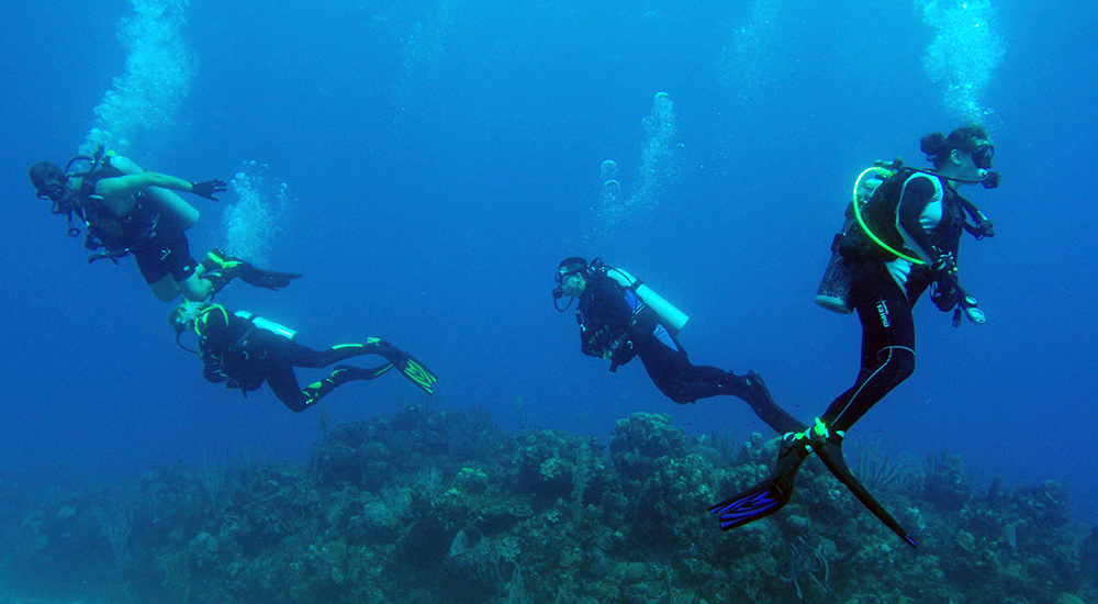
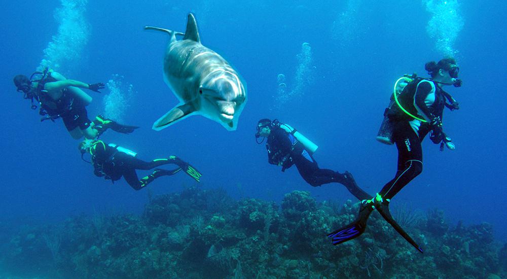
Favorite Result: Dolphin with divers
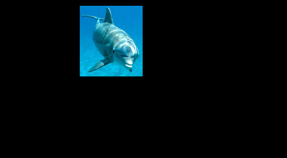
Source
Target
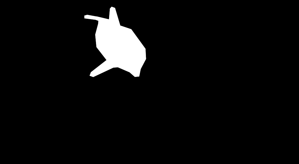
Mask
Naive Blending

Poisson Blending Result
Comparing the naive result to the poisson blending, the seam between the target and source is much better in the poisson blending (in fact, it's barely noticable). It is clear also that the colors of the dolphin itself also changed to match the background better, which makes the image look more natural. This works by using the gradients of the dolphin and applying it to the target image, instead of the absolute pixel values of the dolphin. I didn't need to do anything special for the image, besides just creating an irregularly shaped mask.
Bird in sky
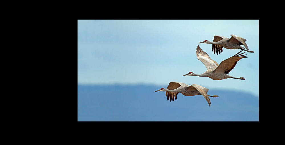
Source
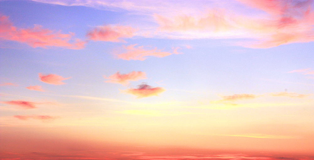
Target
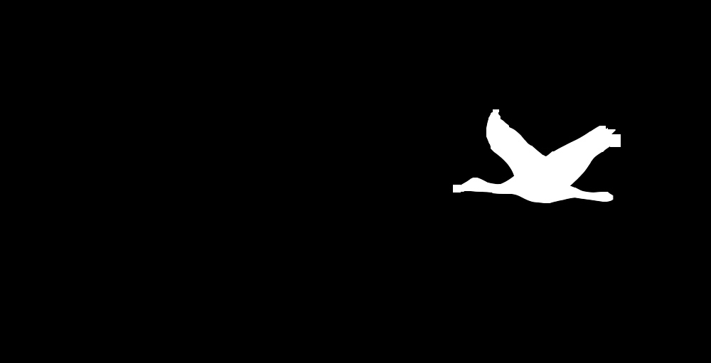
Mask
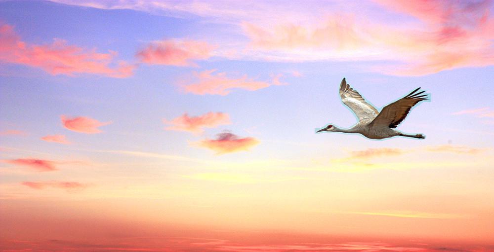
Naive Blending
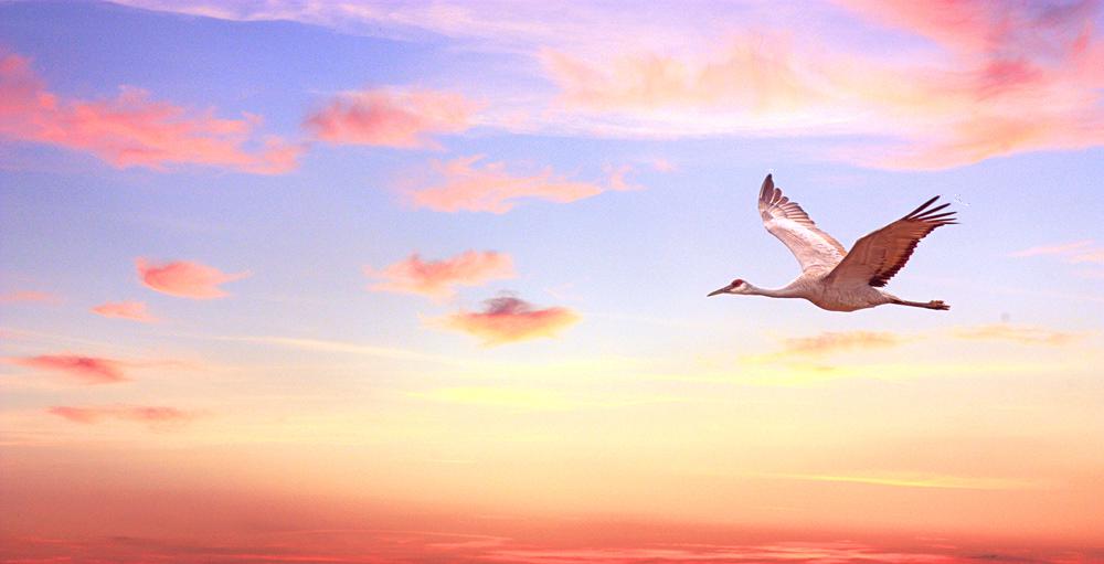
Poisson Blending Result
Failure case: friend with cartoon
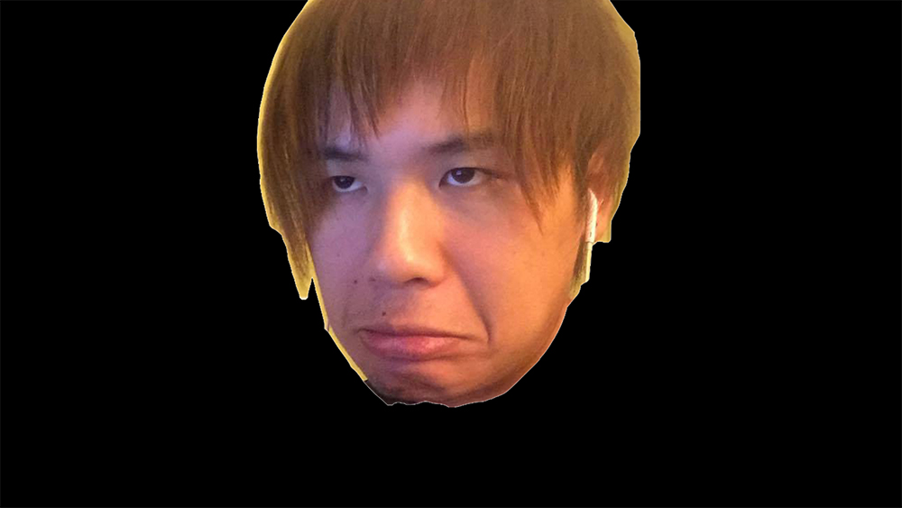
Source
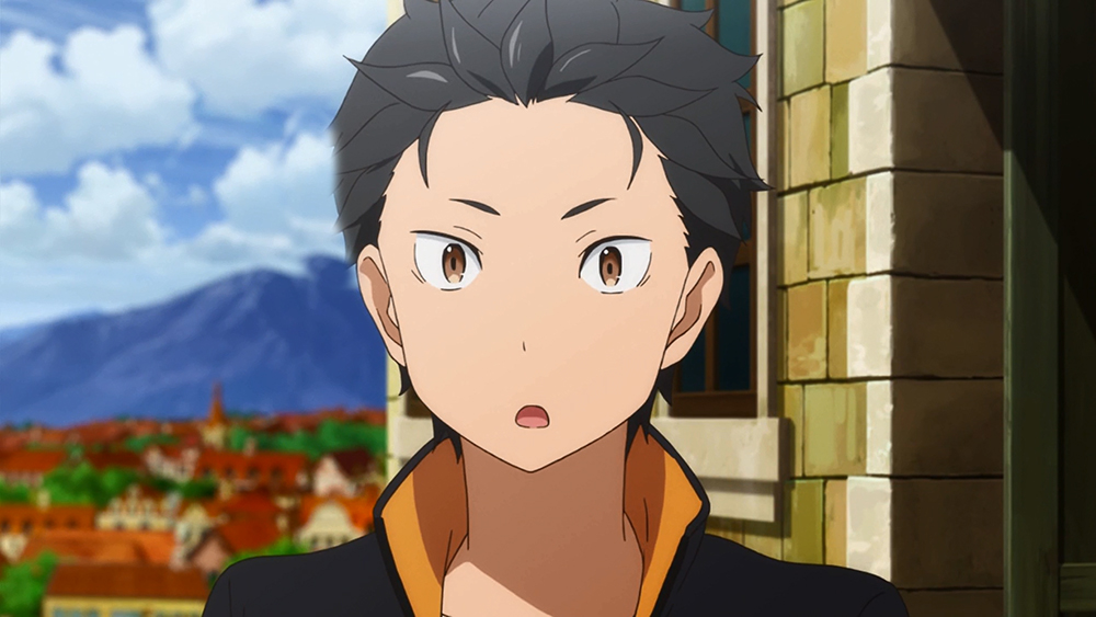
Target
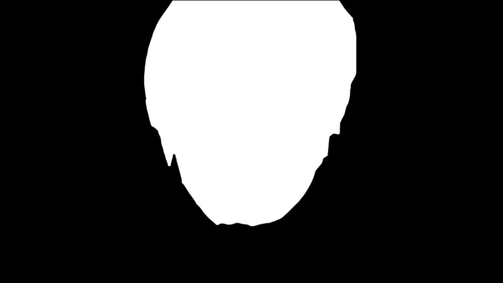
Mask
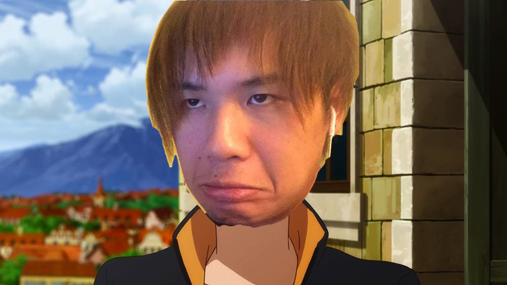
Naive Blending
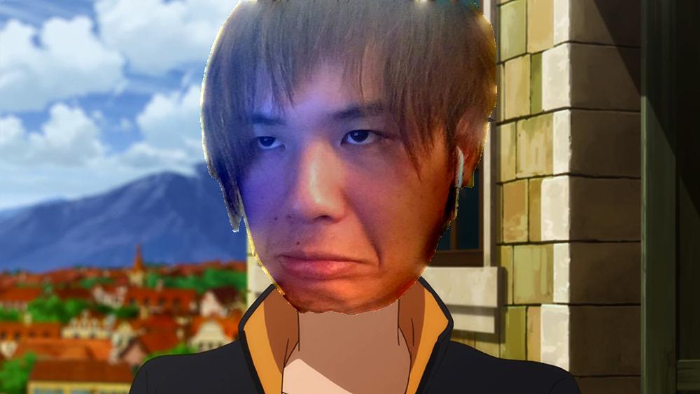
Poisson Blending Result
I believe this one didn't work so well because the backgrounds were just too difference. Moreover, there was a lot of detail in the area I was trying to graft onto which makes the mistakes painfully obvious. Also, the orientation of the faces is not identical which probably increases how wrong it looks as well.
Comparison with other blending techniques:
Source
Target
Mask
Naive Blending
Multiresolution Blending
Poisson Blending
Poisson blending clearly works the best for these two images, because the fact that it uses gradients instead of absolute pixel intensities makes the seam much less noticable. In almost all cases, this will give the best blending result. However, if it is important to preserve the original intensities of the source images, then the other techniques may be more appropriate. I think multiresolution blending is a good compromise between poisson and naive for that specific case.