Project 3
Part 1: Frequency Domain
Part 1.1 Sharpen Images
I picked the original picture of my friend and used the sharpening technique described in class: filter extrat the high frequences of the image (threshold=sigma) and add it to the original image scaled by constant alpha.
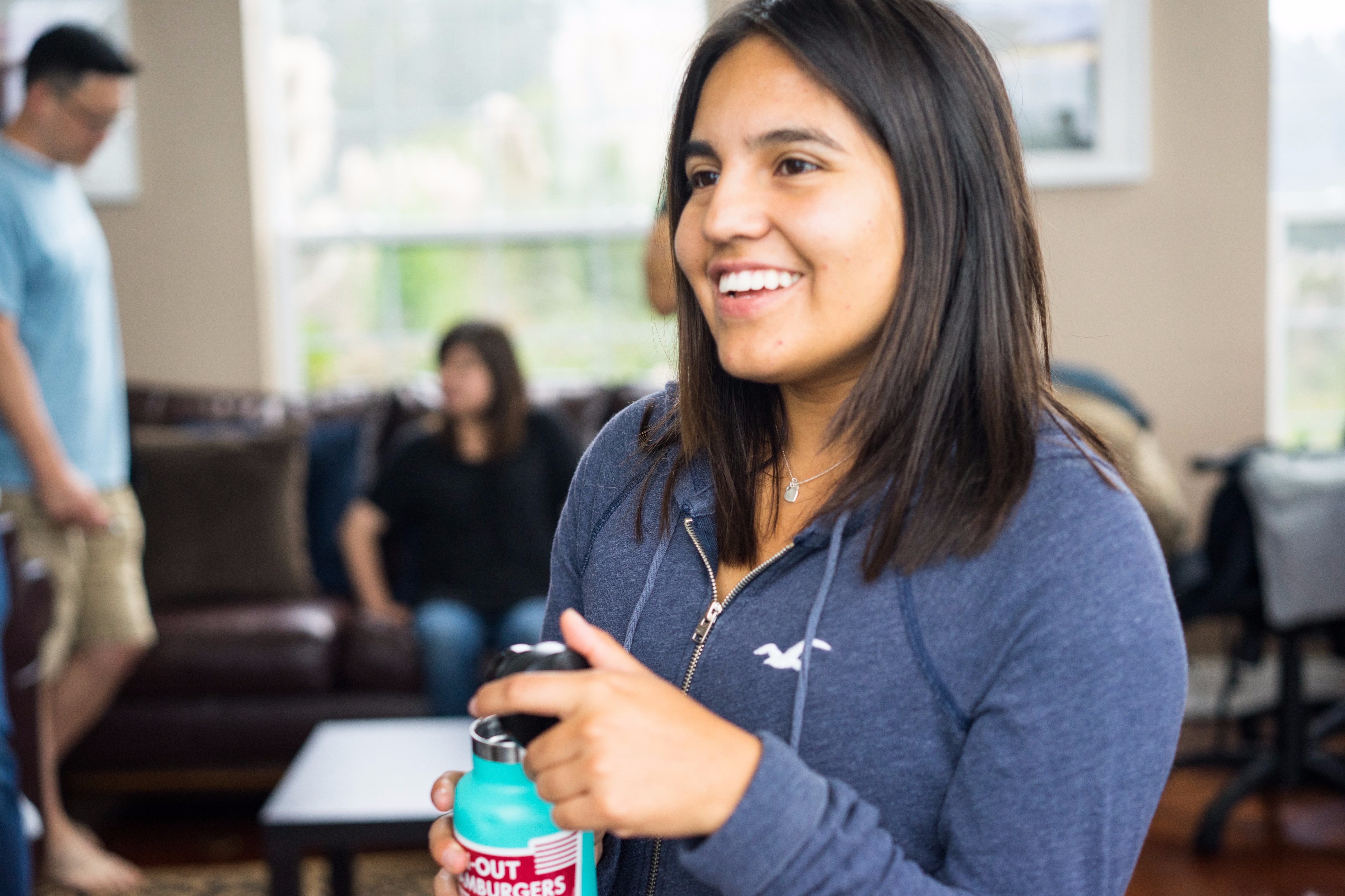 Original
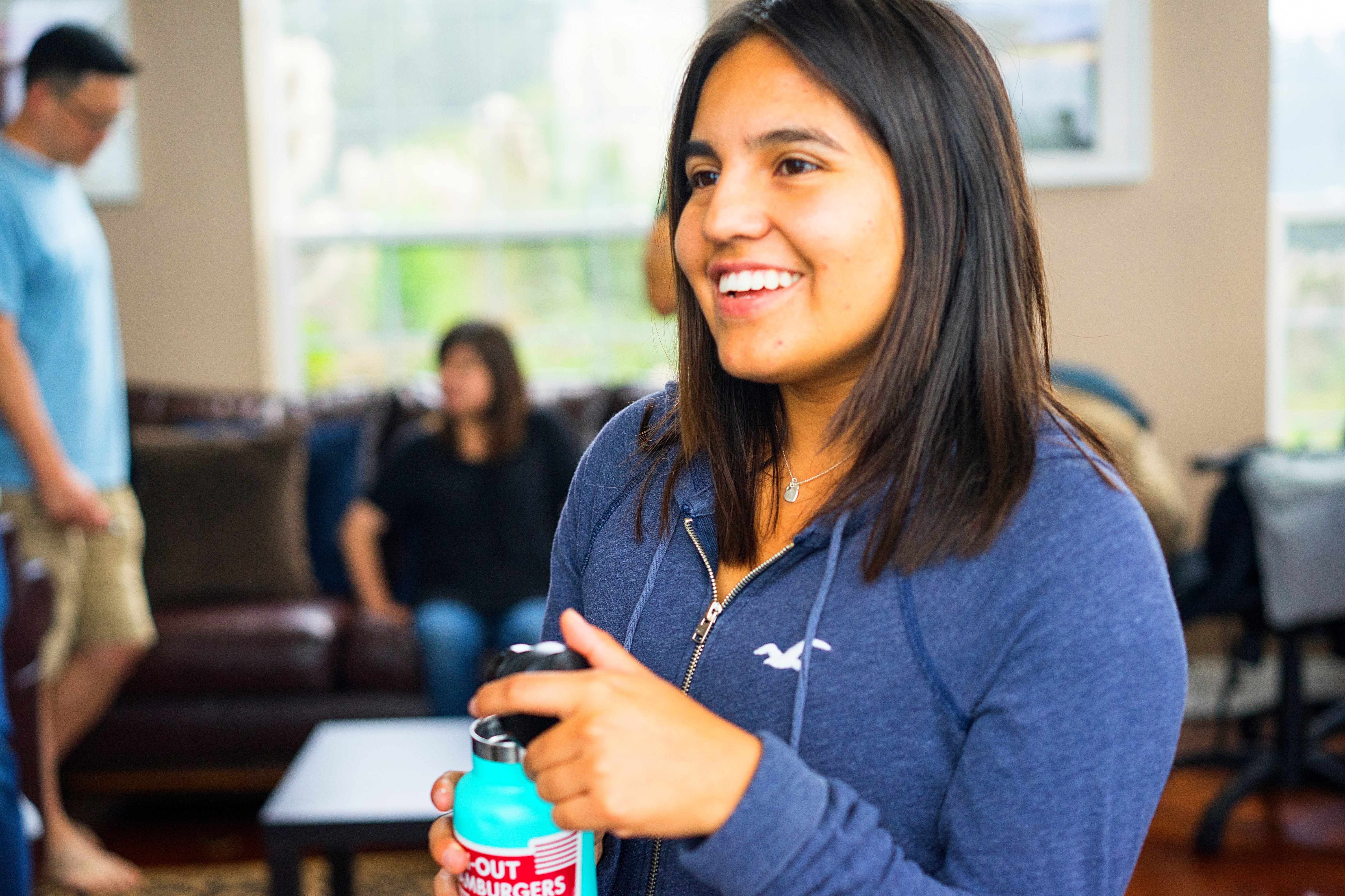 Sharpened (alpha = 0.5, sigma = 5)
 Sharpened (alpha = 0.25, sigma = 5)
Photo Credit: Mica.
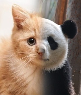
Part 1.2 Hybrid Images
I blended three pairs of images. First I low-pass filter one image and high-pass filter the second image, each with its corresponding threshold sigma. Then I add them together, each weighted with its corresponding alpha.
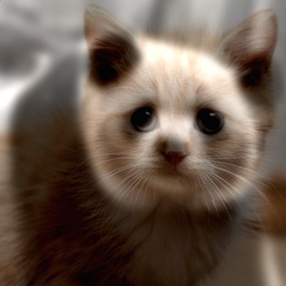 Panda: low (sigma=5, alpha=2)
Cat: high (sigma=100, alpha=0.5)
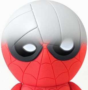
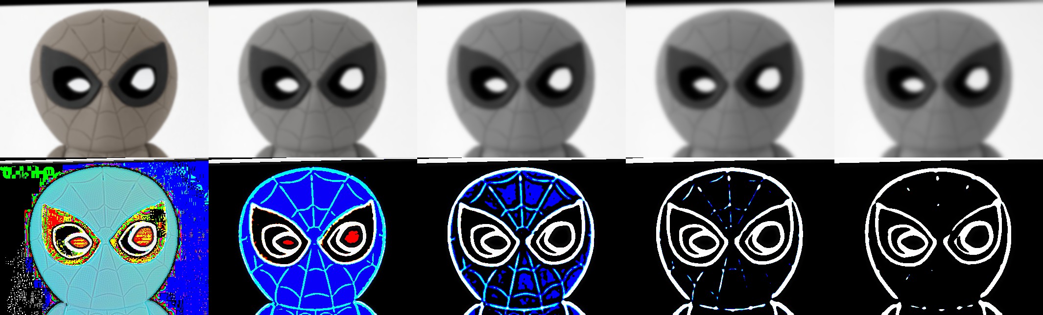
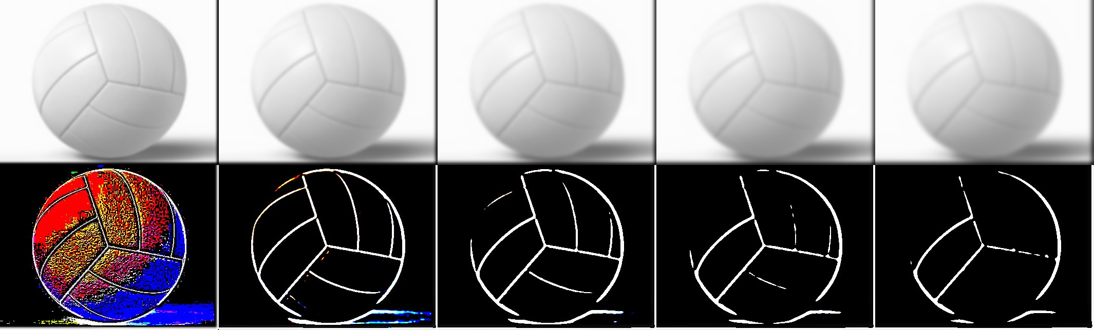
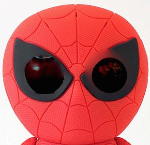
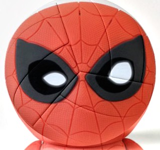 Spiderman: low (sigma=0.5, alpha=1)
Volleyball: high (sigma=20, alpha=1)
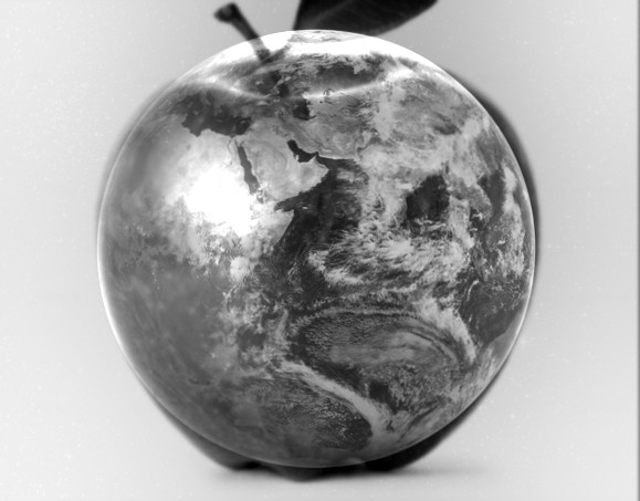
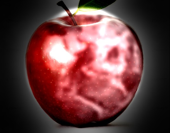
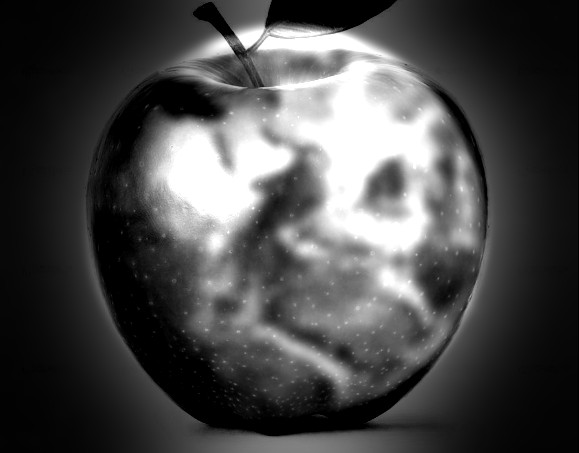
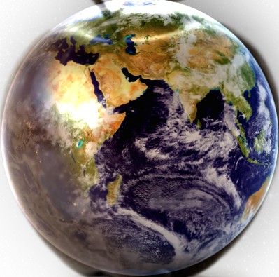 Apple: low (sigma=1.5, alpha=1)
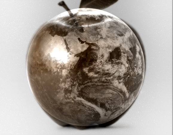
Earth: high (sigma=50, alpha=1)
Failure case: the line of the volleyball crossed the hollow eye of the spiderman.
Following is the illustration of the frequencies of the images at different stages.
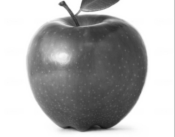
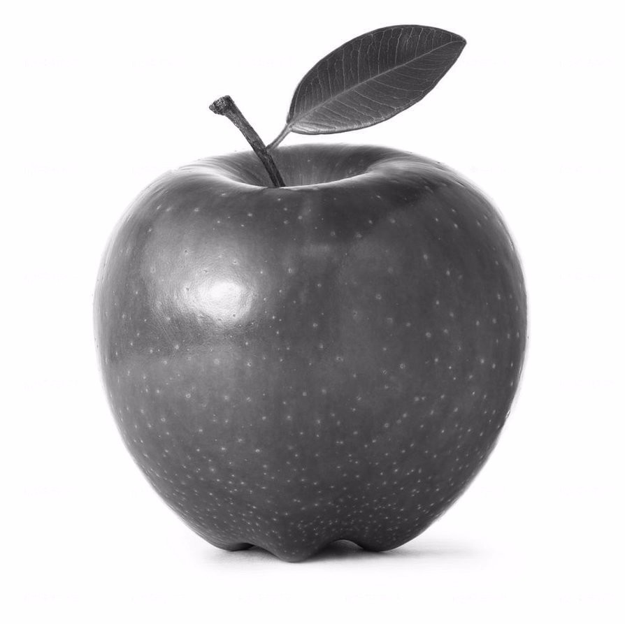 Apple input
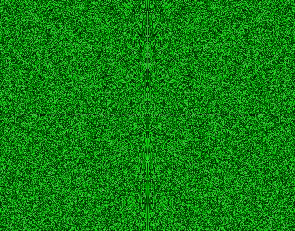
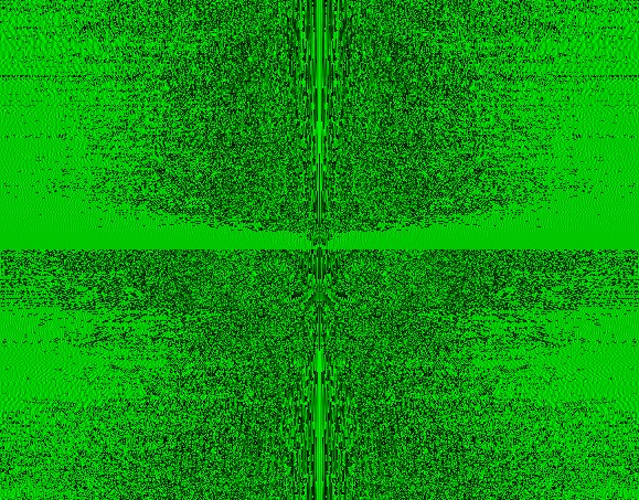 Apple input FFT
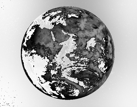
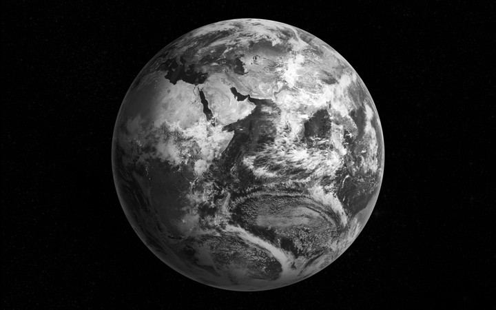 Earth input
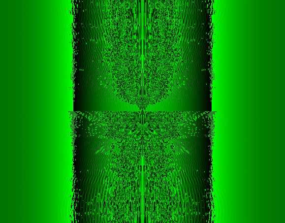
 Earth input FFT
 Apple: low (sigma=1.5, alpha=1.2)
Earth: high (sigma=100, alpha=0.8)
 Apple filtered
 Apple filtered FFT
 Earth filtered
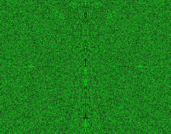 Earth filtered FFT
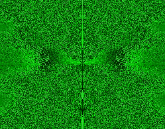 Blended result FFT
Extra Credit: Use Color
It seems that using color for the high-frequency component is much better than using color for the low-frequency component. The previous examples show the results when both components are colored.
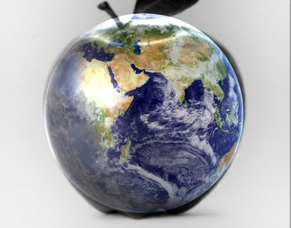 Color high-frequency component (earth)
 Color high-frequency component (apple)
 Color low-frequency component (apple)
 Color low-frequency component (earth)
Part 1.3 Gaussian and Laplacian Stacks
I implemented Gaussian stack by successively applying Gaussian filter using threshold sigma to the previous image until reach level N (e.g. N=5). Laplacian stack is created by subtracting each Gaussian image by the image at the level immediately below it.
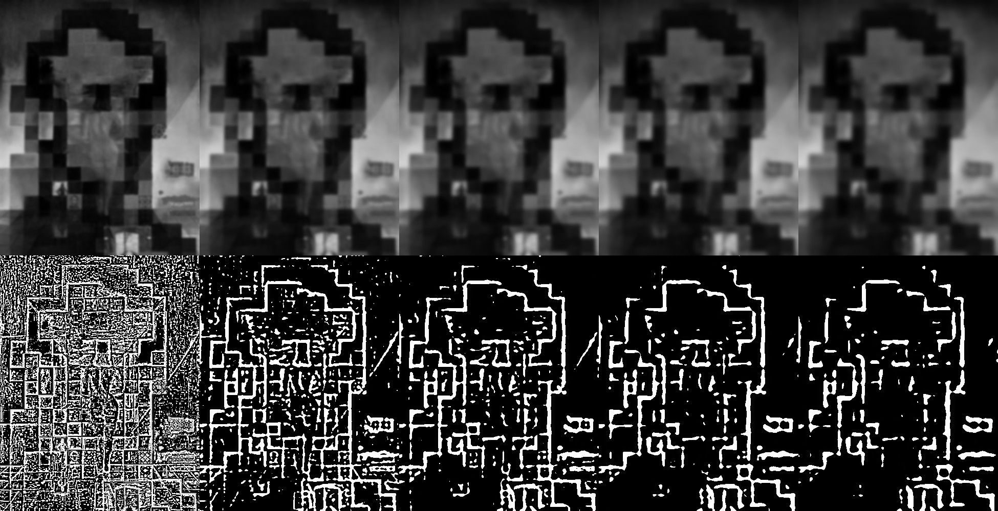 Lincoln (sigma=2, top: Gaussian, bottom: Laplacian)
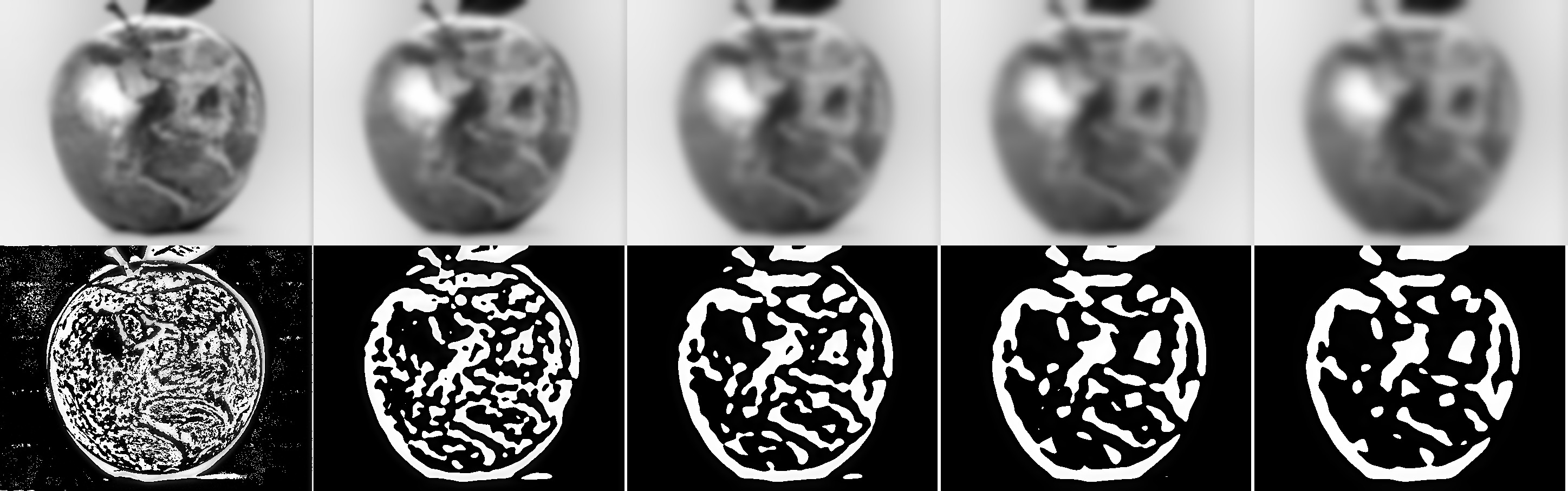 Apple and Earth (sigma=5, top: Gaussian, bottom: Laplacian)
Part 1.4 Multiresolution Blending
I first computed the Gaussian and Laplacian stacks of both input images. Then I created a mask, either manually or using python, which consists of only 1 and 0. Then I create Gaussian stack for the mask. For each level of Laplacian stacks, I mask the input images using the mask on the corresponding level and blend them together. Then I blend the lowest level of Gaussian stacks of the two input images. Then I sum up all the blended images, i.e. the blended Laplacian images and the most blurred Gaussian image.
 Cat and Panda
 Volleyball and Spiderman
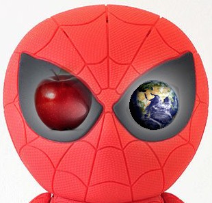 Spiderman, Apple and Earth
Below are the Laplacian stacks that I computed, as well as the masked input images that created it.
 Spiderman
 Volleyball
 Blended image
Extra Credit: Use Color
See above.
Part 2: Gradient Domain Fusion
Part 2.1 Toy Problem
Denote the width and height of the image as w and h, respectively. I first created a matrix A of size (w*h, w*h). Each row represents the function to use to calculate the gradient at that pixel. For the 4 corner pixels, its gradient is 2 * its intensity - the intensities of the two neighbors. For the pixels on the edges, their gradient is 3 * its intensity - the intensities of the three neighbors. For the inner pixels, the gradient is 4 * its intensity - the intensities of the four neightbors. The top left pixel retains its intensity, as suggested by the spec. In this way, I formulate a least square system and reconstructed the image.
 Original
 Reconstructed
Part 2.2 Poisson Blending
In this part, we use poisson blending to blend a source image into a target image seamlessly.
I picked the original picture of my friend and used the sharpening technique described in class: filter extrat the high frequences of the image (threshold=sigma) and add it to the original image scaled by constant alpha.
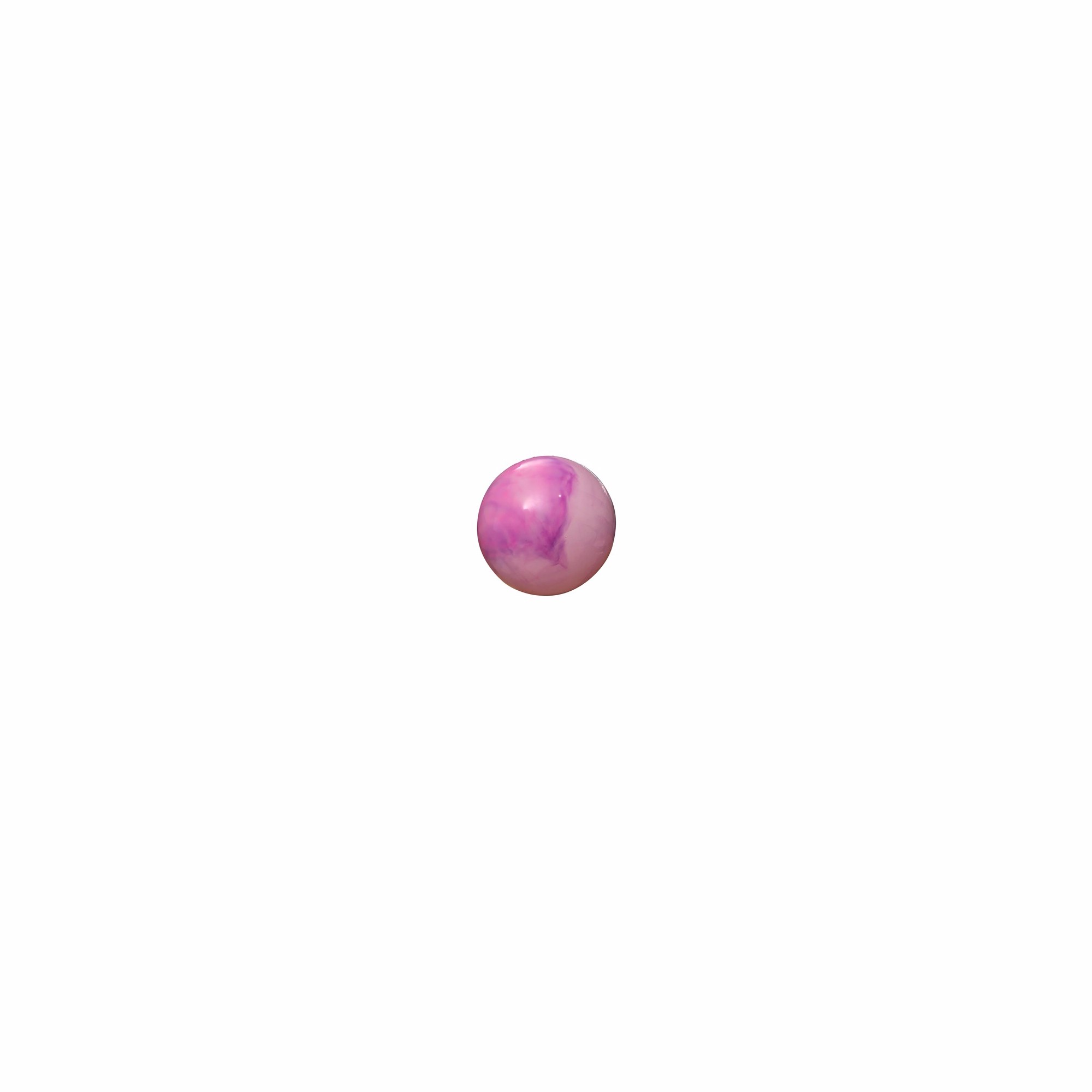 Marble
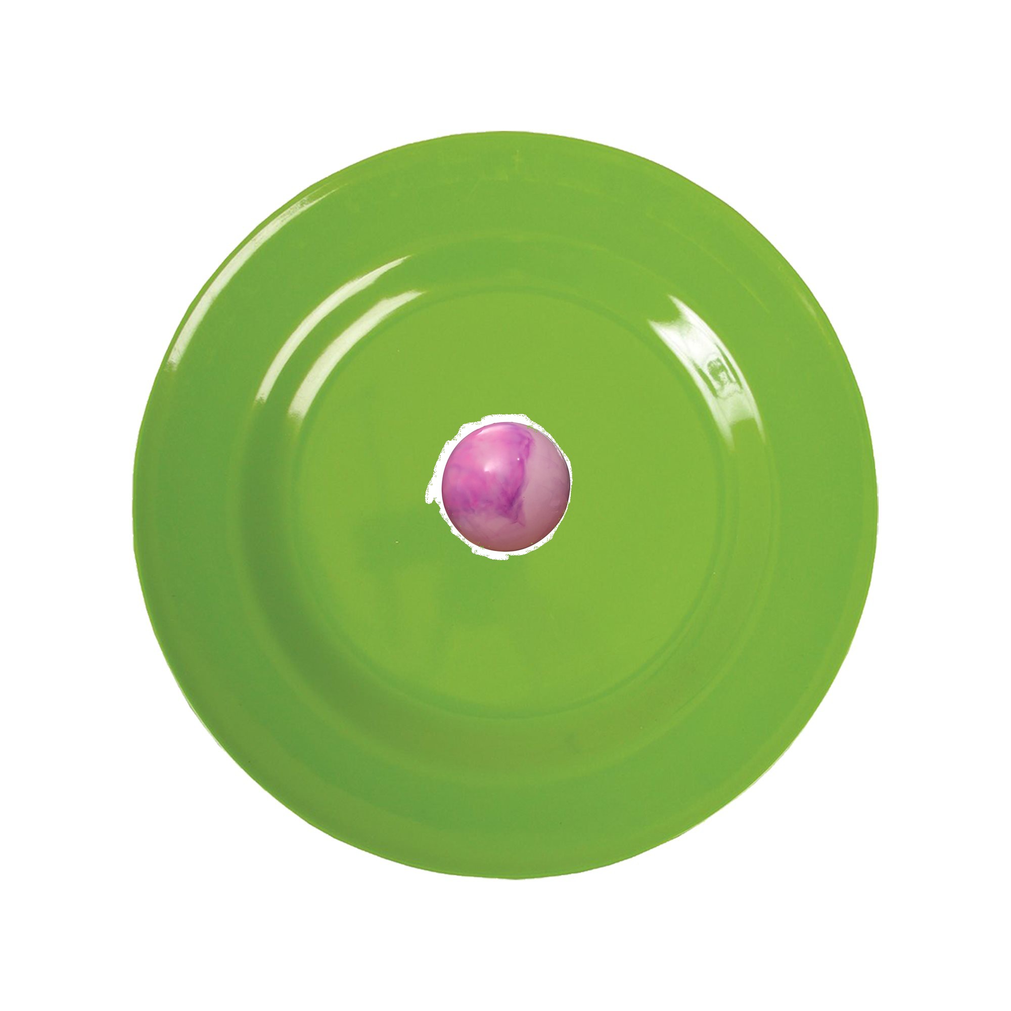 Directly Copied
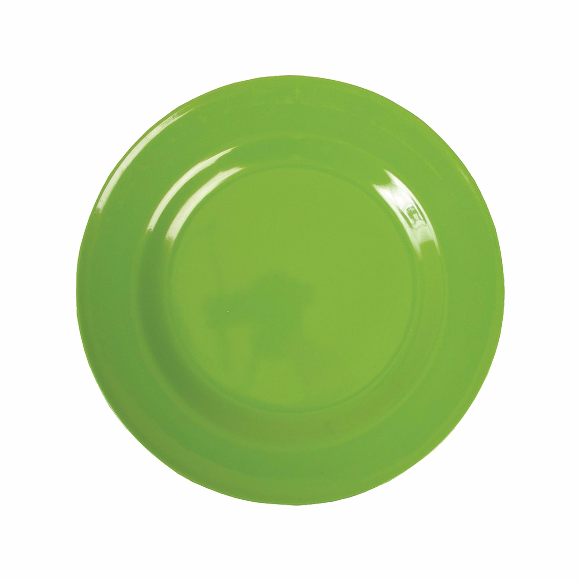 Plate
Plate
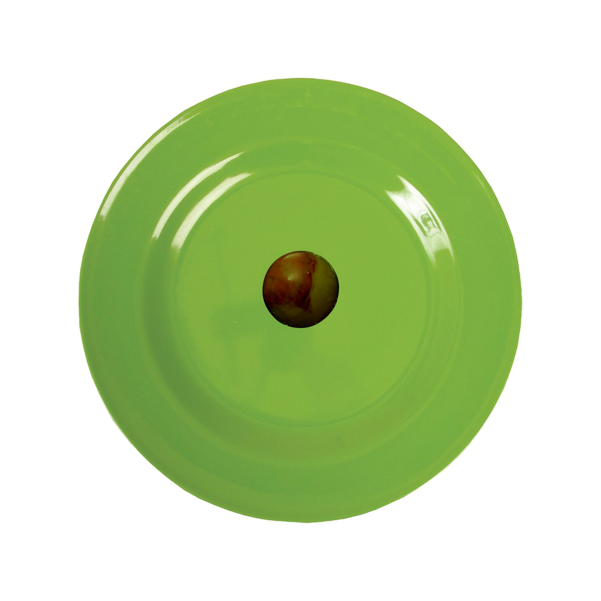 Poisson Blended
More Results:
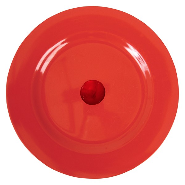 Red marble
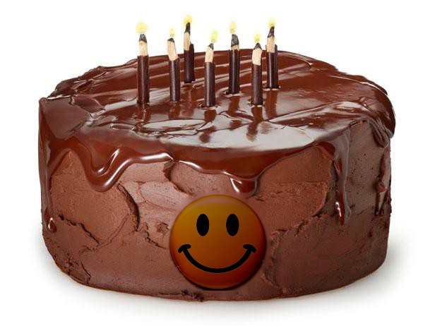 Cake with smile
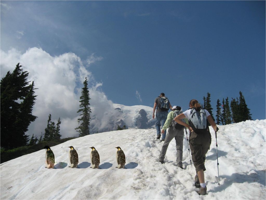
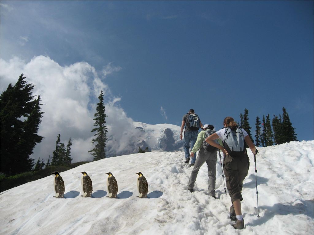 Four penguins
Failure case: The smiley face retained its yellow color because the original picture border was white (so poisson blending retained the difference between the color of the face and its surroundings). The leftmost penguin was added by poisson blending. The head of the penguin had "bleeding" effect because the target image has very different gradient from the source image around that area.
Contrast between multiresolution blending and poisson blending.
Multiresolution
 Poisson
Neither looks good probably because the masks confused the poisson algorithm of the color.
Extra Credit: Mixed Gradients
Contrast between using source gradient and using mixed gradient.
Source blending
 Mixed blending
Extra Credit: Color2Gray
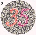 Original
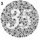 Gray
Gray