CS194-26 Project 3: Fun with Frequencies and Gradients!

YiDing Jiang

Overview

In this project we will explore several techniques to blend images using mathematical tools such as fourier transform, image frequencies, and sparse matrix techniques.

Part 1: Frequency Domain

1.1 Warmup

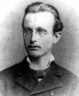
I create a high pass filter by convolving the image with a gaussian filter, then subtracting the result from the original image to extract edges. Then I add the high frequency component back to the original image to enhance the edge features. The sigma of the gaussian filter is 8 and the scaling factor for the edge alpha is 1.

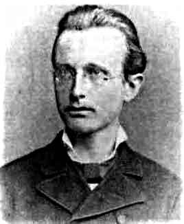Original Planck	Sharp Planck

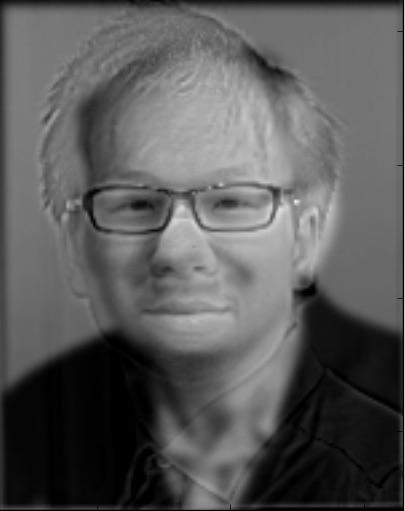
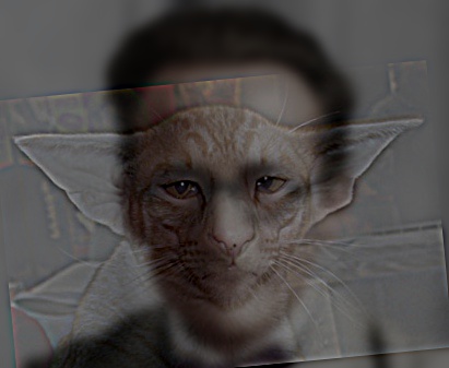
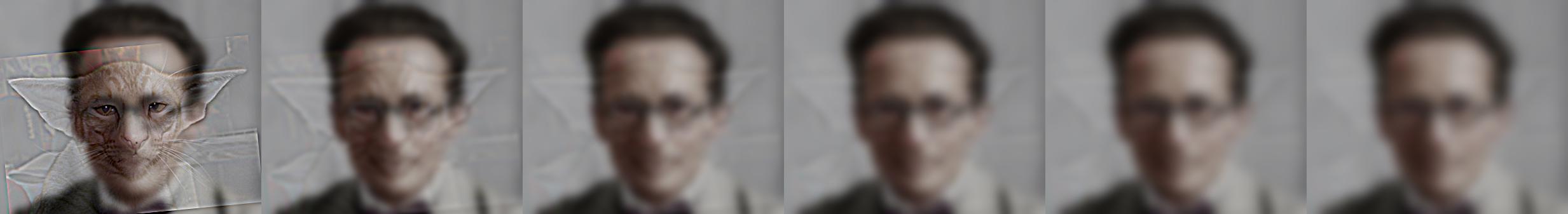
1.2 Hybrid Images

Hybrid images are the result of combining high frequency components and low frequency components from two different images. The two components are obtained through convolving one with a high pass filter (1.1) and the other with a low pass or gaussian kernel. The results are averaged or weighted average depending on the nature of the two images. The sigma of the gaussian filters are chosen experimentally as they may be different depending on the images.

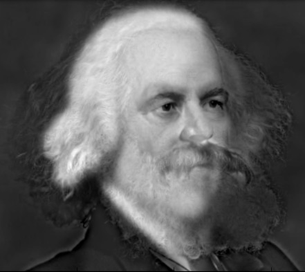
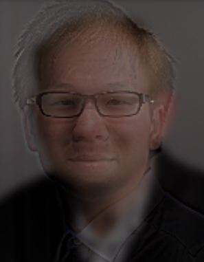
Quantum CS194-26 Staff	Capitunism (fail)	Erwin Schrodinger and a sad Cat

If you cannot tell, the second image is a blend of Adam Smith and our favorite Karl Marx. This one did not quite work out because Marx's beard does not fade away at distance no matter how I tuned the hyper-parameters. Marx's beard is a extremely prominent feature and it has a very different colors and textures from its surrounding. As the result, no matter how the hyper-parameters are chosen, it always stands out. The mechanics of this image at some level requires the brain to do template matching and finish the picture. The beard makes recognizing Adam Smith much more difficult. I guess sometimes things just don't mix well together.

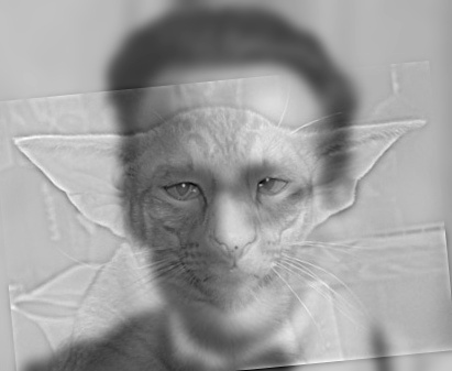
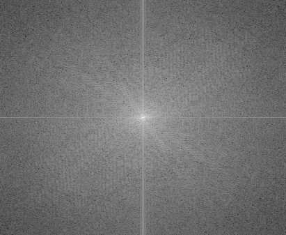
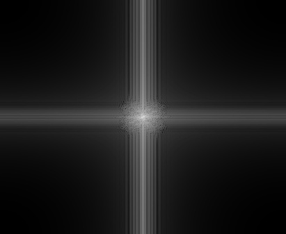
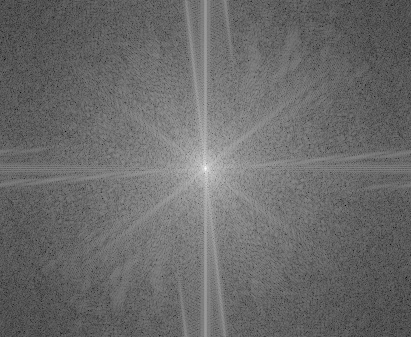
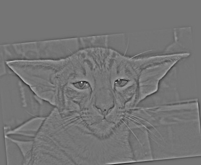
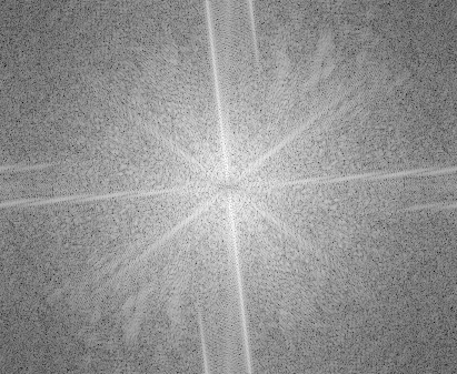
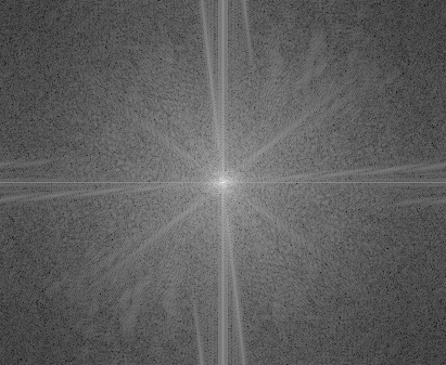
Below is the fourier analysis of Schrodinger and cat:

Type	Original Image	Original Fourier Transform	Filtered Image	Filtered Fourier Transform
Low Frequency
High Frequency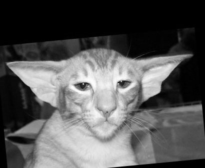
Hybrid

Colorized

We can use colors to make these hybrids more interesting:

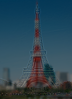Schrondinger's cat (colorized)	Alyosha Zhu	Why is it red now?

The color of the high frequency components are usually faded away during the filtering, so the colors of the low frequency components will always be very visible; this examples are down with color in both sources, but the result with only colors in the low frequency image look qualitatively very similar, unless the high frequency source has very dominant frequency in one channel (e.g. starry night below).

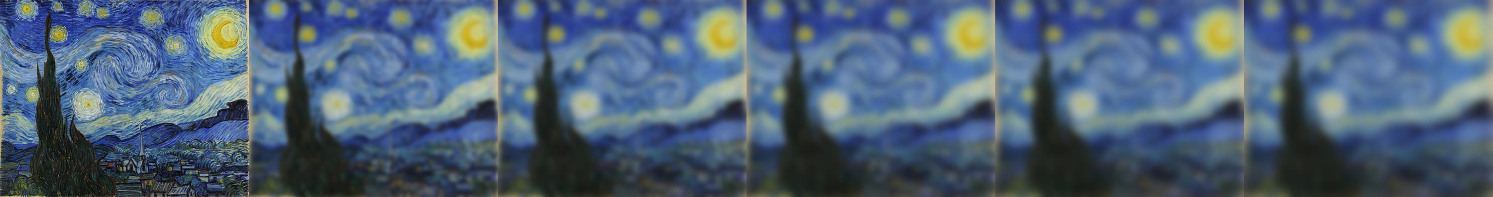
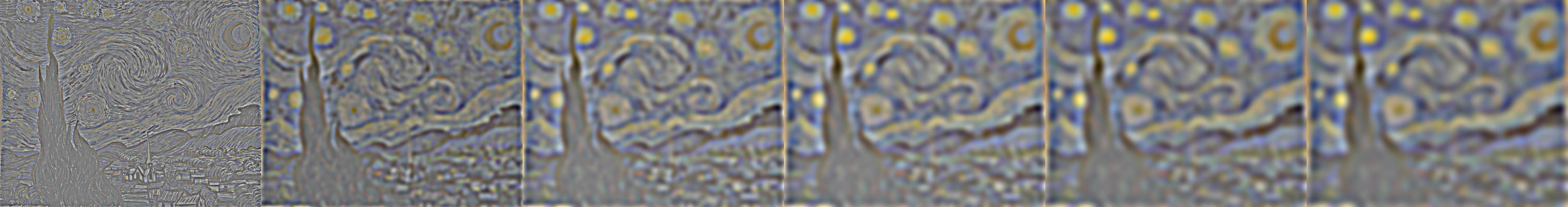
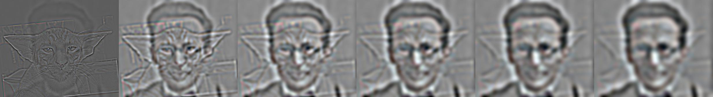
1.3 Gaussian and Laplacian Stacks

A Gaussian stack is created by keep convolving the same image with a gaussian filter without downsampling. A Laplacian stack is the difference between the layers of a Gaussian stack. Here the sigma is 4. The Laplacian pyramid is rescaled to [0, 1] for visualization.

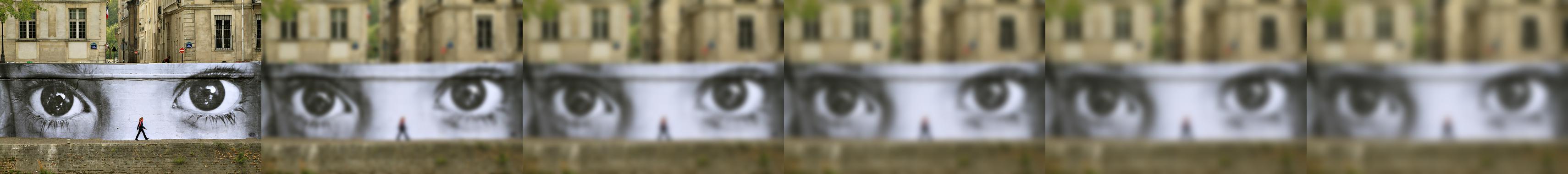
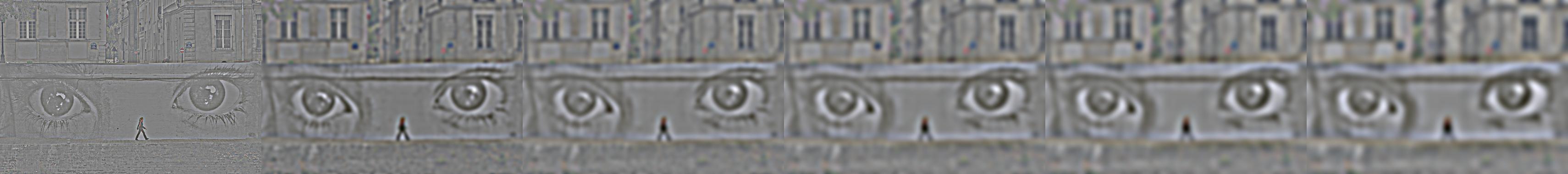
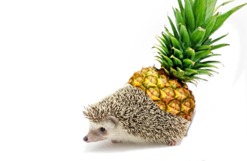
1.4 Multiresolution Blending

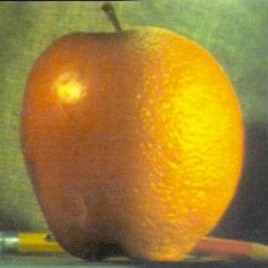
With the Gaussian and Laplacian stacks above, we can perform multiresolution blending be mixing each layer of the Laplacian stack with different amount to create a visually seamless blend such as the orapple above. Formally, this is done by creating a Gaussian stack for a binary mask. We then point-wise multiply the binary stack with corresponding levels of one laplacian stack and 1 minus the binary mask with the other laplacian stack. At the end we sum the levels together to create a seamlessly blended image.

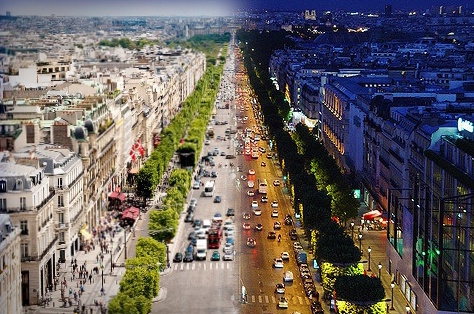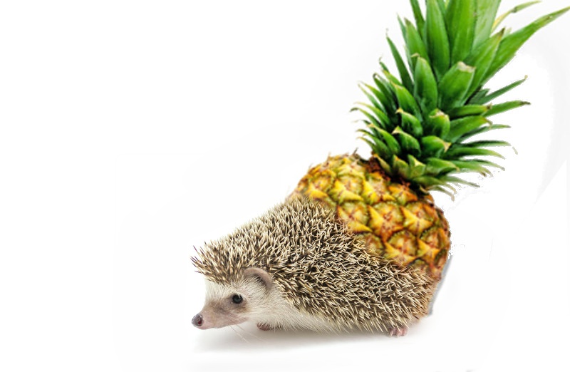Avenue des Champs-Élysées	Pinehog/Hedgeapple?

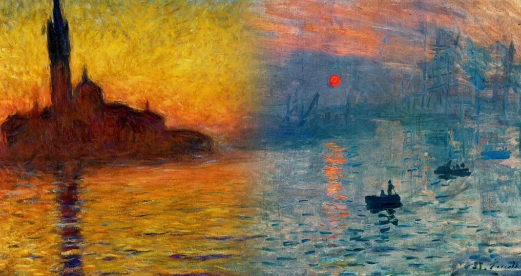"Impression, Sunset in Venice" -- Claude Monet

Below is the process of the creation of the amalgamation of animal and fruit:

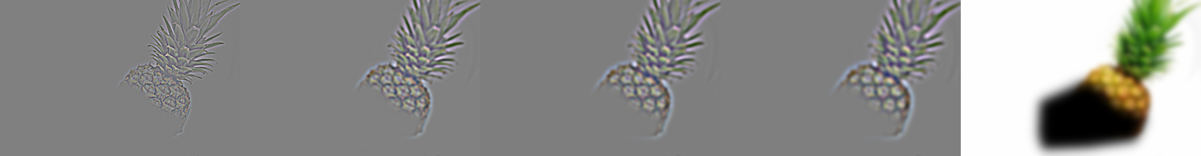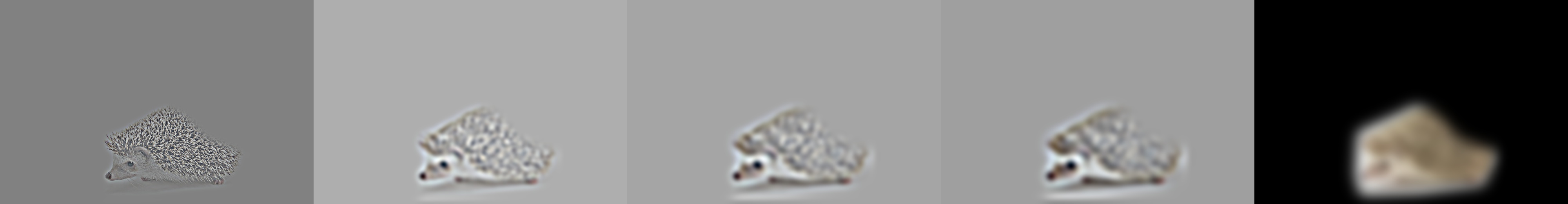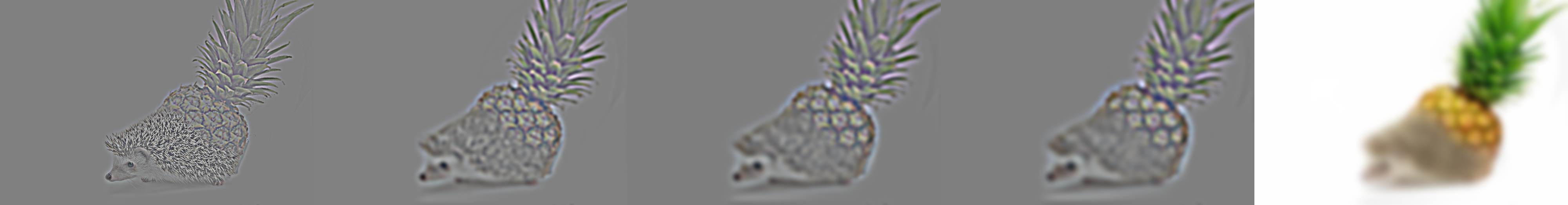They had to be mutilated for science :(

Part 2: Gradient Domain Fusion

An alternative to blending with Laplacian and Gaussian stack is to blend with image gradients. The theory is that we are much more perceptible to changes to gradients rather than the color itself; therefore, suppose target T is the image where we try to blend the source image S into, the strategy is to match the gradient of V, the new pixel values, within the mask, M, as closely to the origin S as possible while adding boundary constraints on V such that at the boundary of M, its gradient is close to that of the T. These operations can be done by setting up a sparse constraint matrix A, a reconstruction vector x, and a target gradient vector and value b, and then perform linear regression with Ax=b.

2.1 Toy Problem

This is toy example that recover the same image by matching the x and y gradient of the original image and the pixel value of the top left pixel.

Original	Reconstruction

The l2 norm of the residual between the two image is 0.0013533, which means the two are extremely close to each other in the euclidean space.

2.2 Poisson Blending

Here, we use a slightly more sophisticated methods to solve the following optimization problem:

This optimization problem can be reformulated as a linear regression problem where we try to match the total gradient of S (sum of a pixel's gradients with its 4-neighborhood) and the boundary constraints outside of the mask. This operation can be captured by a Laplacian filter.

In practice, we first naively blend the two image two gether through multiplying with the mask and add together. Then we create a matrix that is h*w by h*w where h and w are the dimension of the resulting image, where each row represents the constraints on one pixel. For each pixel, if the matrix is in the mask, we set its corresponding location in its row in the matrix to 4 and its 4 neighbors to -1. We set its corresponding location in b to its total gradient in S. If the pixel is outside the mask, we simply set its corresponding entry in A to 1 and set its entry in b to the pixel value of the same pixel in T. Solving for and reshaping the optimal x yields a poisson blended image.

Target	Source	Naive Blend	Poisson Blend

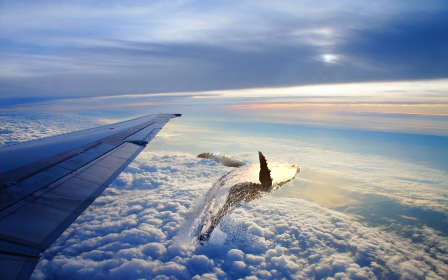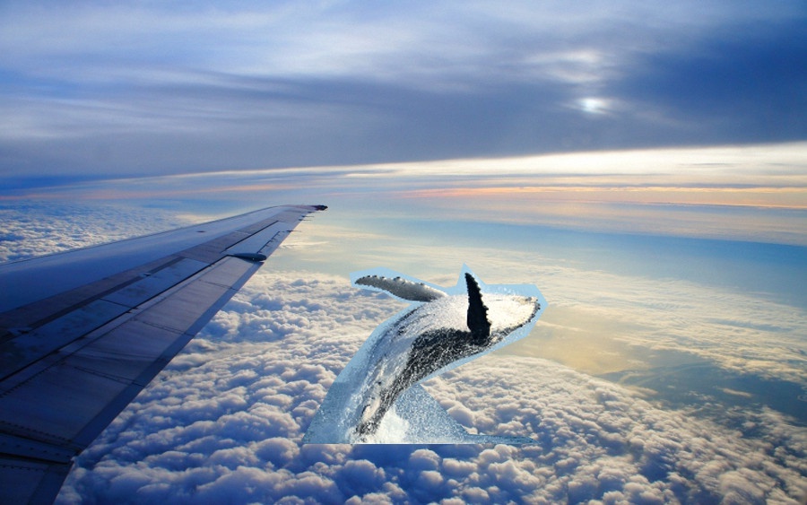
Below are some results:

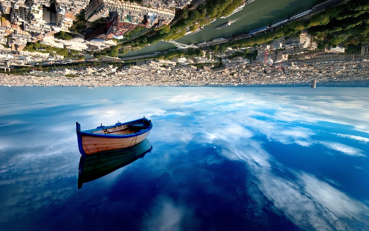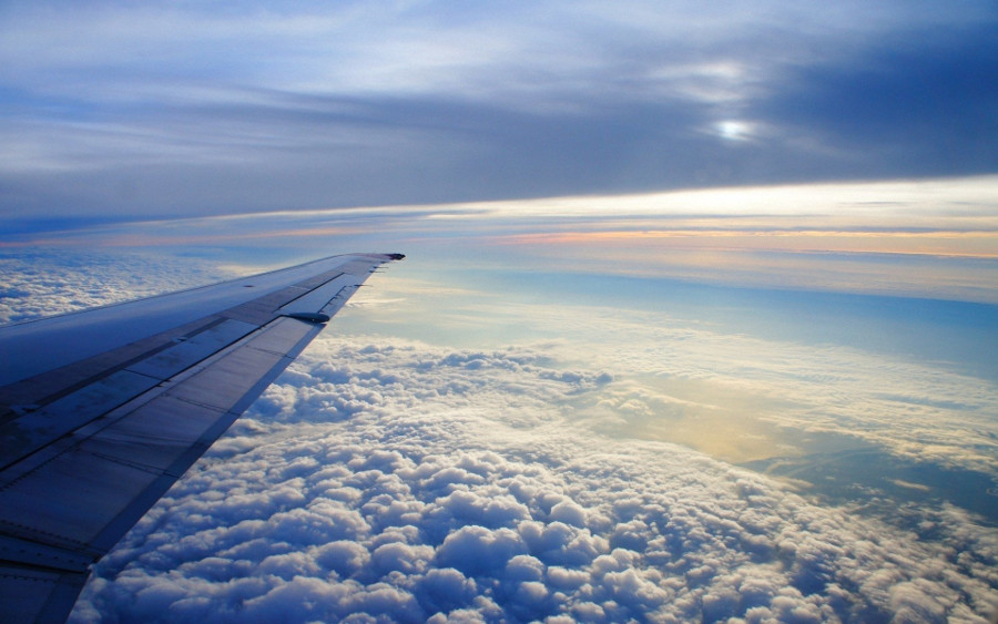
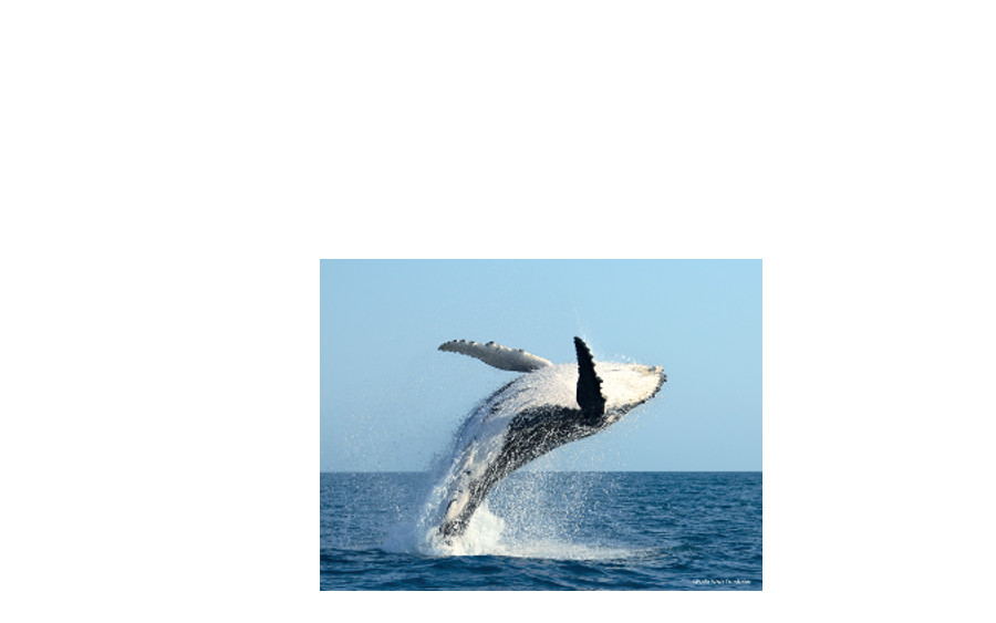
Whale Watching	Boating Over the Seine
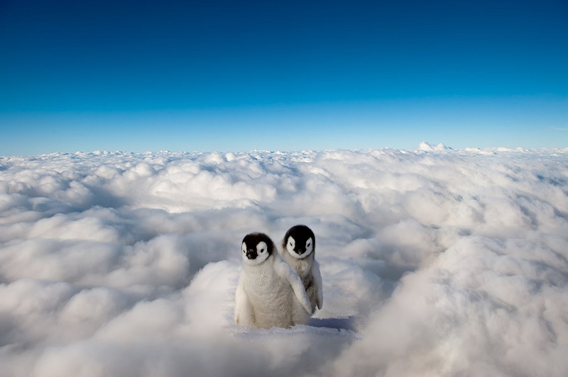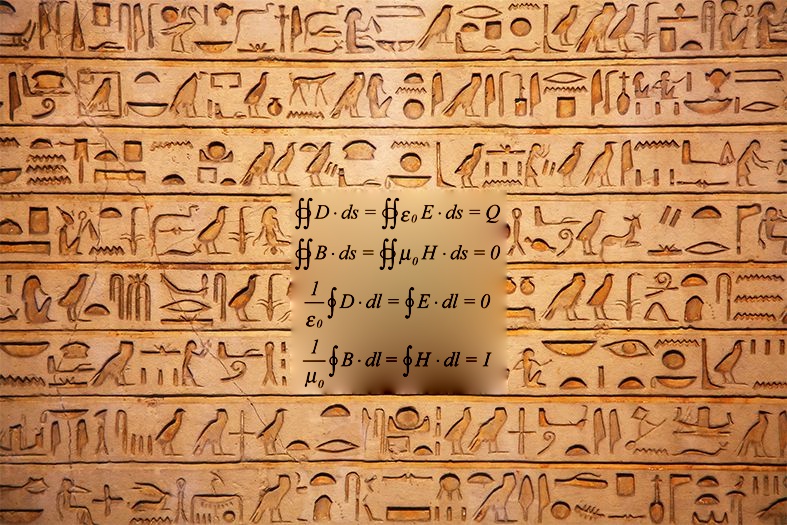Something I know will work	I know this wouldn't work

As you can see the attempt to write Maxwell's equation onto a wall of Hieroglyphs failed because the texture of the Hieroglyph are very different from the pure white background of the equation. Simply trying to match the gradient of the source will produce the blurred and texture-less color gradients in the image, which does not look natural at all.

We can now try to blend pineapple and hedgehog from earlier with Poisson blending and compare the results:

Naive	Laplacians blending	Poisson blending

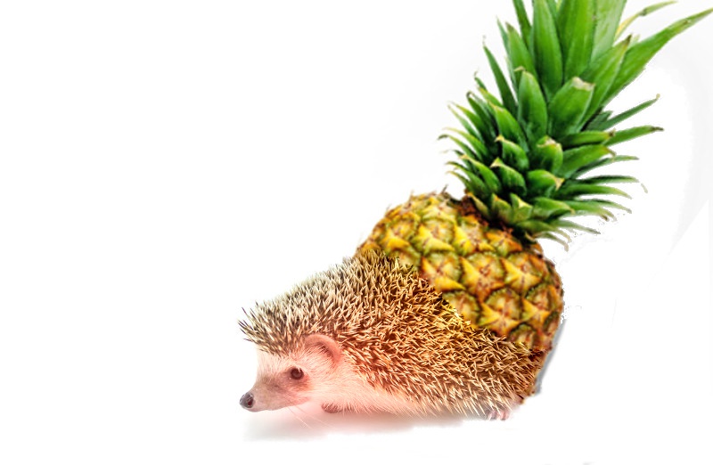We see that Poisson blending makes all the spikes of the hedgehog more orange and closer to the color of the pineapple and makes pinehog more orange/redder. However, when dealing with very complicated feature mismatch around the seam, Laplacian actually does better than Poisson as we can see in the pinehog's case.

This is because Laplacian blends images at different frequency levels independently which better captures texture, whereas Poisson Blending uses minimizing l2 norm as objective, which means it's good as blend the average gradient changes but less capable at mixing textures. Therefore, when matching color of the overall image is more important, we should use Poisson blending. When we care more about smooth transition between different textures we should use Laplacian.

Mixed Gradients

To address the problem for blending writing, we can use mixed gradient where we match the gradient with larger gradient from S and T. This way, we can capture prominent textures from the target domain even if it's inside the mask.

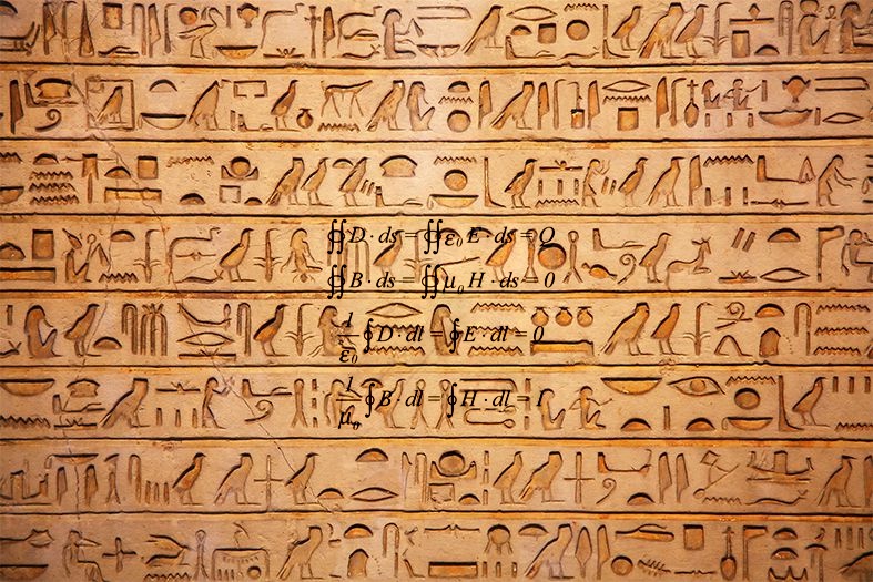Poisson Blending	Mixed Gradient Blending

We see it successfully captures both the equation and the Hieroglyphs.

Final thoughts

This project was very entertaining. I learned that display every step helps a lot. Also I spent way more time looking for appropriate images than coding... Fun stuffs :)