Part 1: Frequency Domain
1.1 Warmup: Image Sharpening
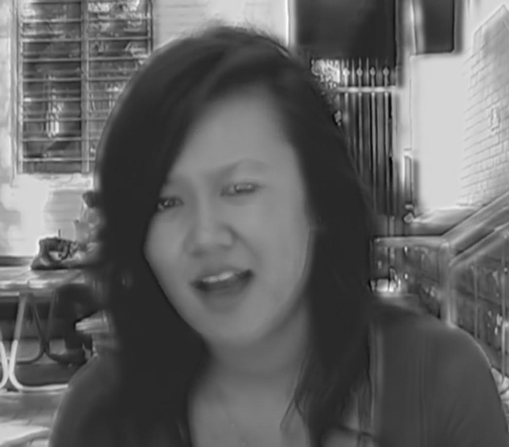
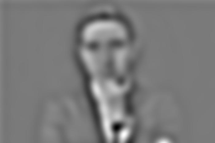
Original Image (Greyscale)
Laplacian Image
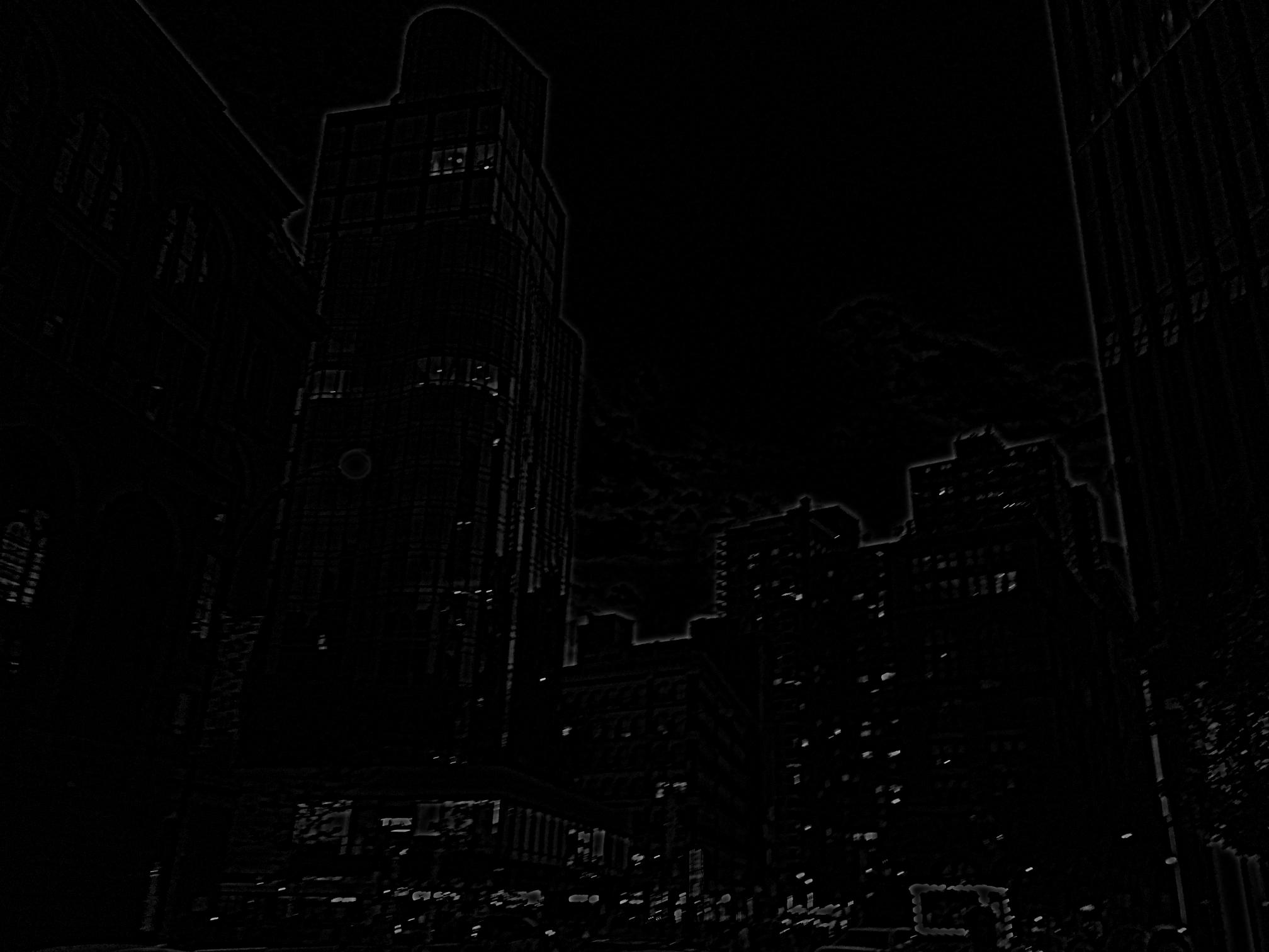
Image Sharpened
Original image vs sharpened image.
1.2 Hybrid Images
Did she just wink at me?
High Freq
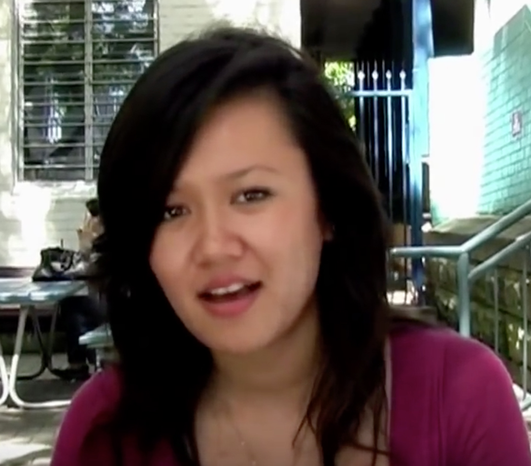
Low freq
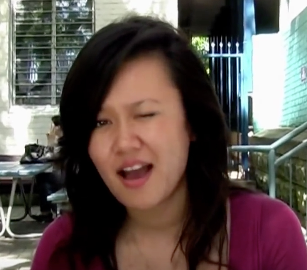
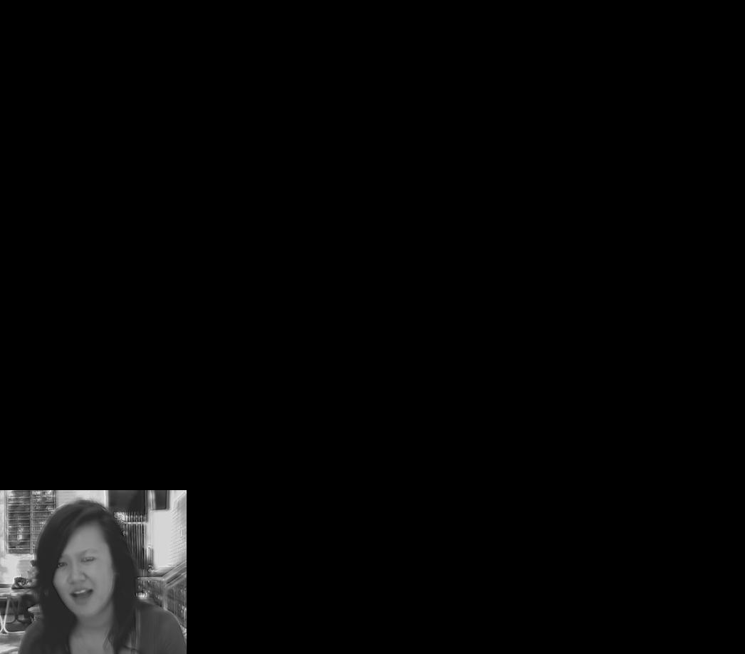
Hybrid up close
Hybrid (at a distance)
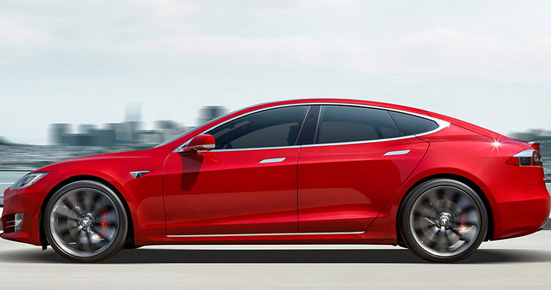
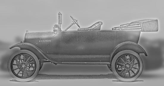
Model T and Model S
High Freq
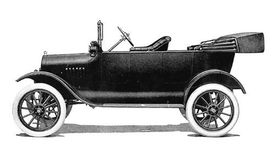
Low freq
Hybrid up close
Hybrid (at a distance)
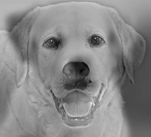
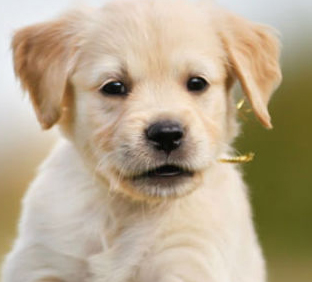
Doggo and Pupper
High Freq
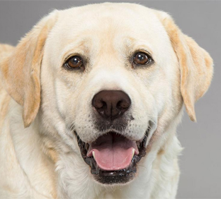
Low freq
Hybrid up close
Hybrid (at a distance)

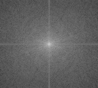
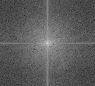
Fourier Analysis of Doggo and Pupper
Doggo in Frequency Domain
Puppy in Frequency Domain
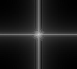
High frequencies of Doggo
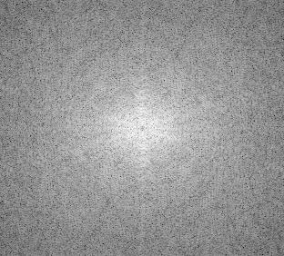
Low frequencies of Pupper
Composite
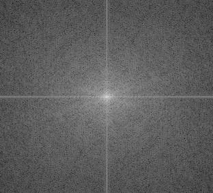
We can observe the properties of the frequency domain based on these results. For the high pass fiter,
we can see a noticable black dot in the center of the image. If we increase the size of the low pass filter used
to create the high pass filter, we can control the size of that center dot. Inversely, the low pass filter produces
a frequency representation with very few values as you move away from the center, as expected.
What's nice, however, is that the Hybrid image has a nice even distribution, similar to that of the unfiltered images
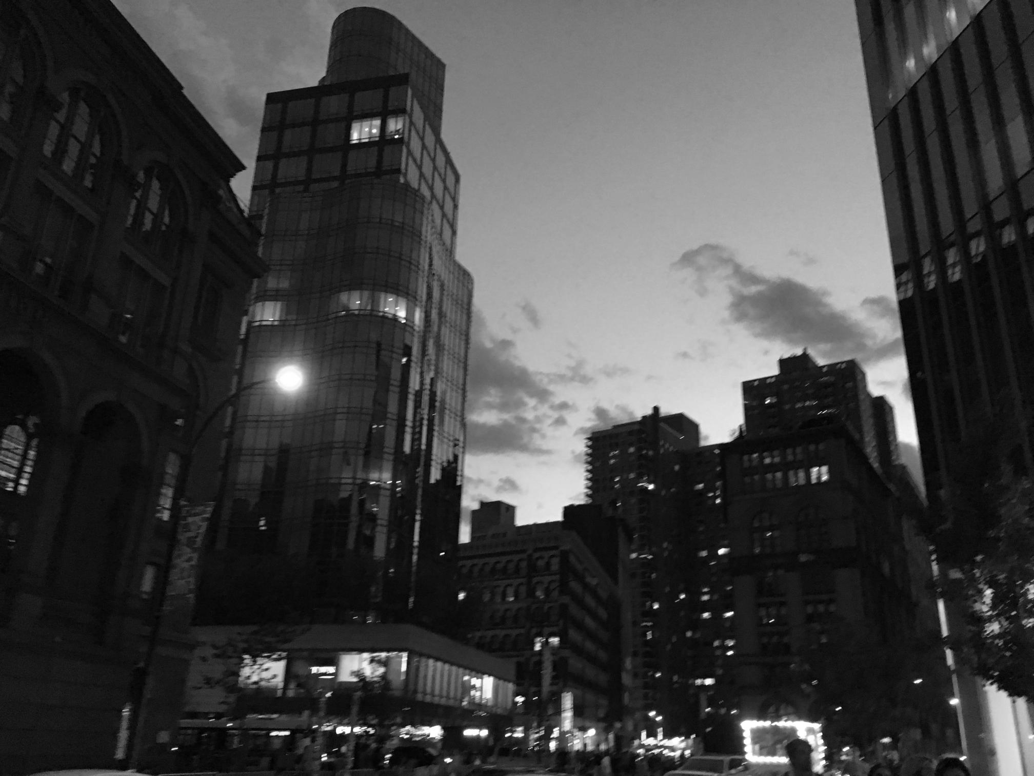
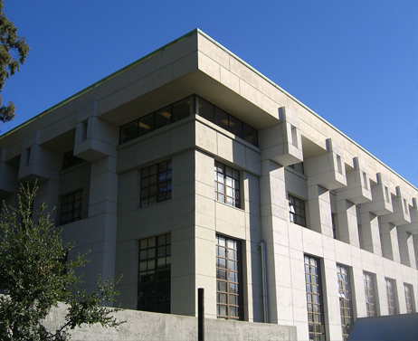
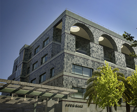
Cory and Soda (Failure Case)
High Freq
Low freq
Hybrid up close
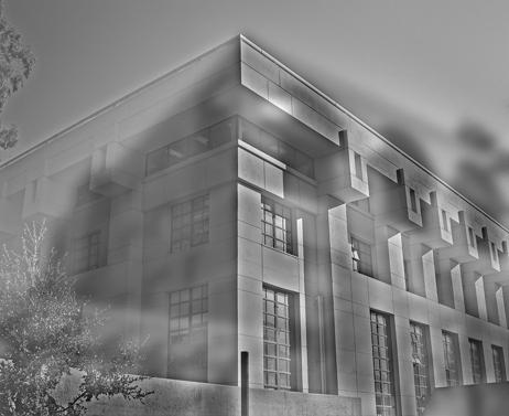
Hybrid (at a distance)

As you can see in the blended image, it's fairly easy to distinguish the Soda even when occluded by
Cory. This is because the occlusion is not full and the angle of hte buildings do not line up, leaving
a large area of the high frequency without a background. This was discussed as a failure case within
Olivia et. al.
Multiresolution Blending
No blending
Seamless blend
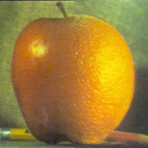
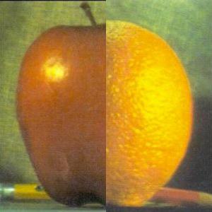
The magical Oraple
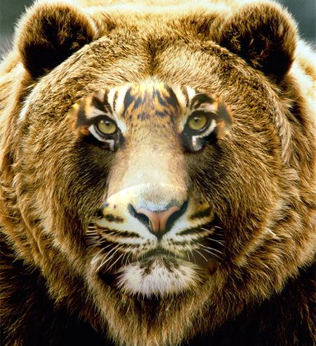
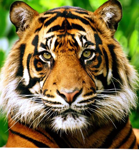
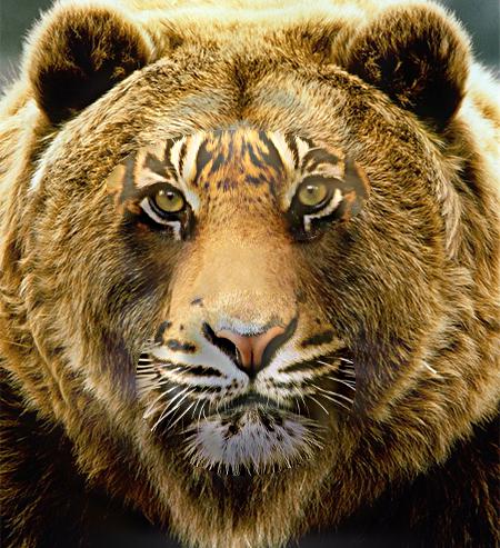
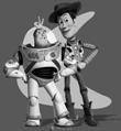
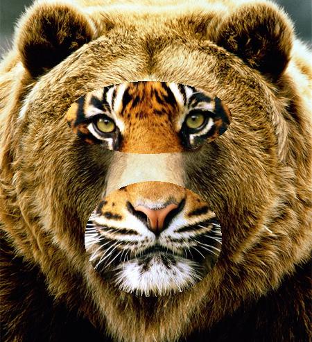
BearTiger
Source Image 1
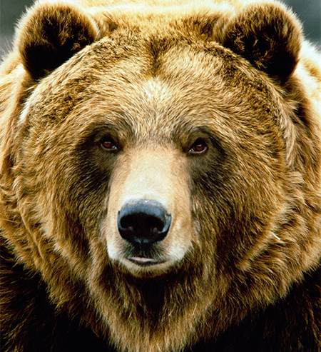
Source Image 2
Naive copy

Blended Image
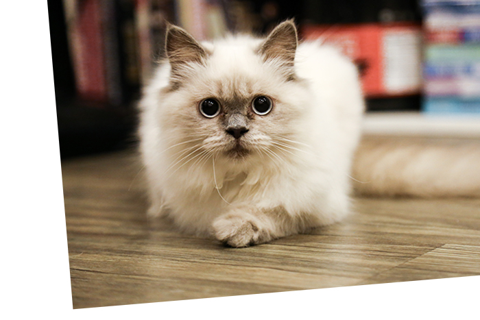
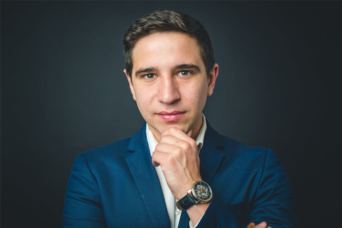
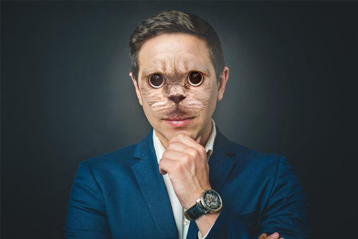
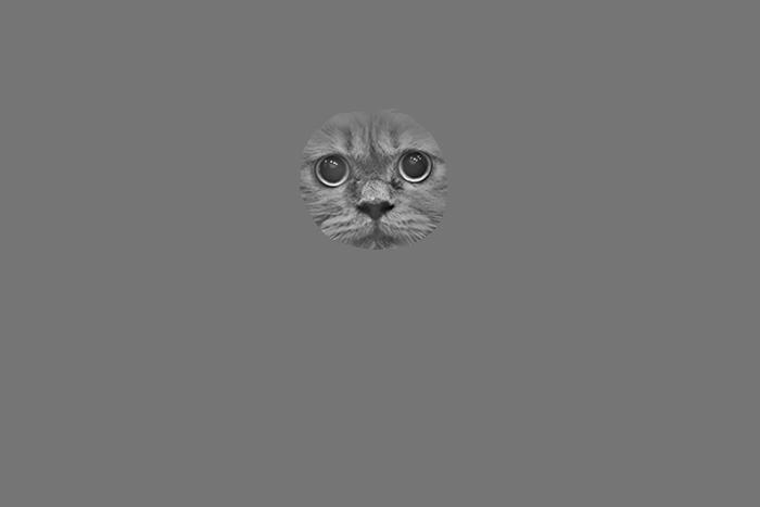
Catface
Source Image 1
Source Image 2
Naive copy
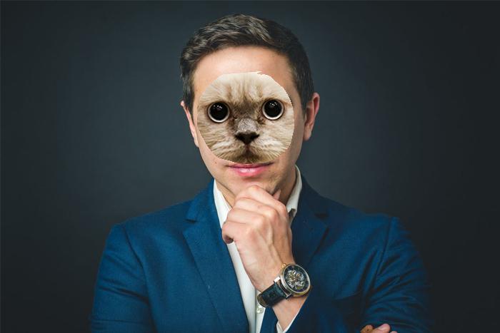
Blended Image
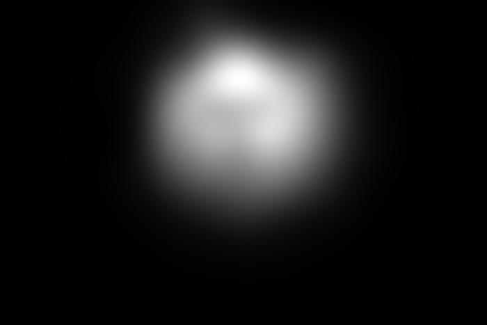
High Frequencies
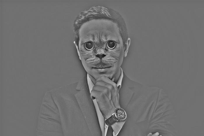
Medium Frequencies
Low Frequencies
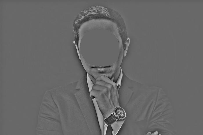
Analysis of the different frequencies of the masked image of the human.
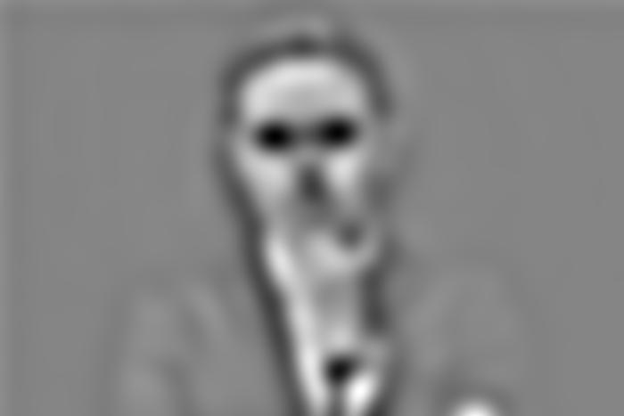
High Frequencies
Medium Frequencies
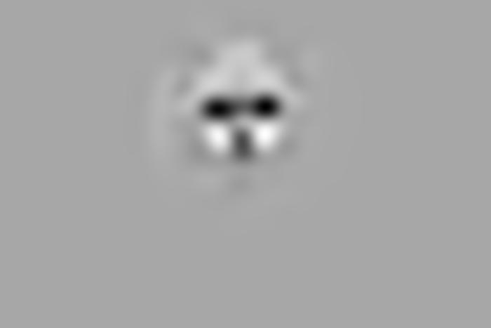
Low Frequencies
Analysis of the different frequencies of the masked cat image. As you can see,
the mask starts to bleed at lower frequencies, incorporating the information from those levels more.
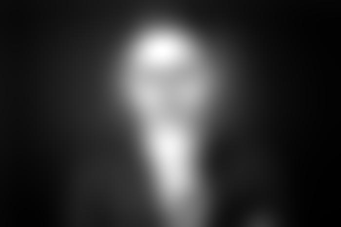
High Frequencies
Medium Frequencies
Low Frequencies
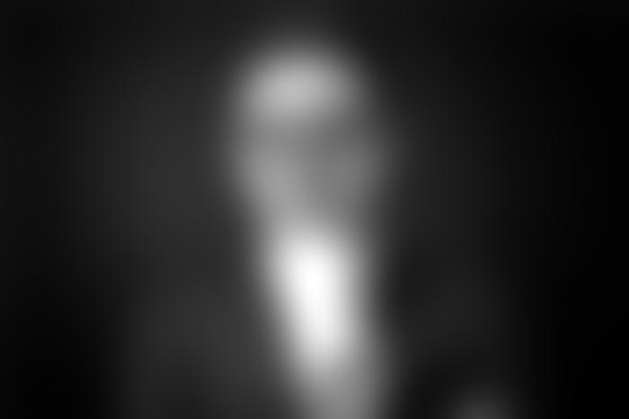
Analysis of the different frequencies of the masked image of the human.
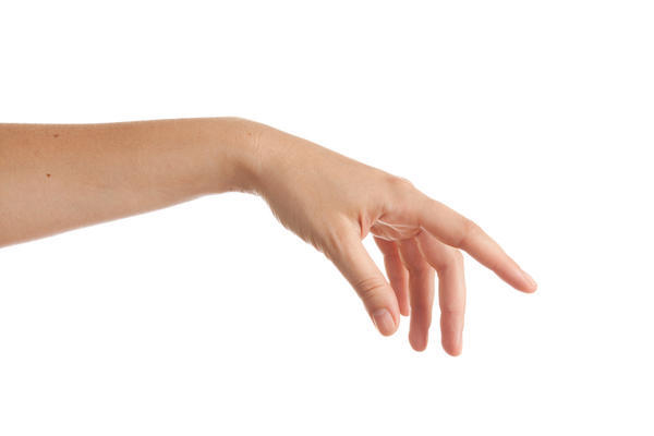
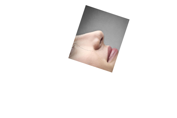
Hand-nose (failure case)
Source Image 1
Source Image 2
Naive copy
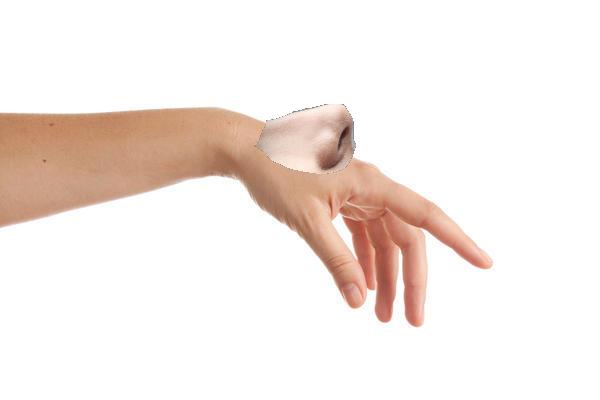
Blended Image
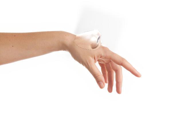
This failure case likely occurred because frequency domain blending softens the boundary of the mask then
effectively takes the weighted average in the higher frequencies of the image. With all the white space in the
masked region, the algorithm picks up way too many misleading color clues and creates an unintended faded
image.
Part 2: Gradient Domain
Toy Problem
Toy Image

Single "color" constraint
Reconstructed Image
Poisson Blending
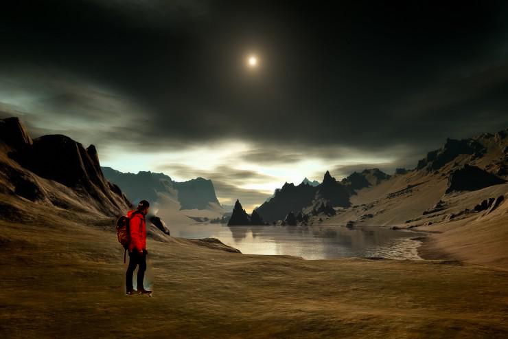
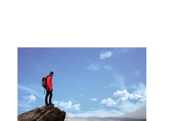
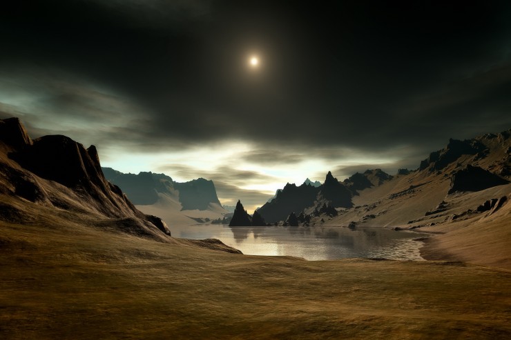
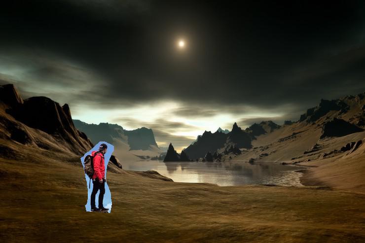
On an alien planet
Foreground Image
Background Image
Naive Copy and Paste
Blending result
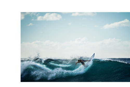
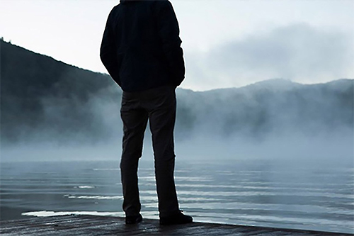
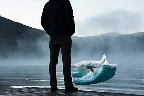
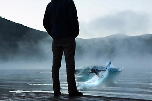
Mini-surfer on a calm lake
Foreground Image
Background Image
Naive Copy and Paste
Blending result
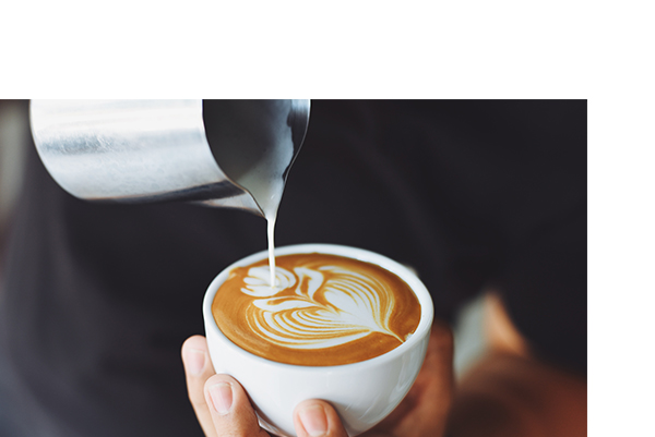
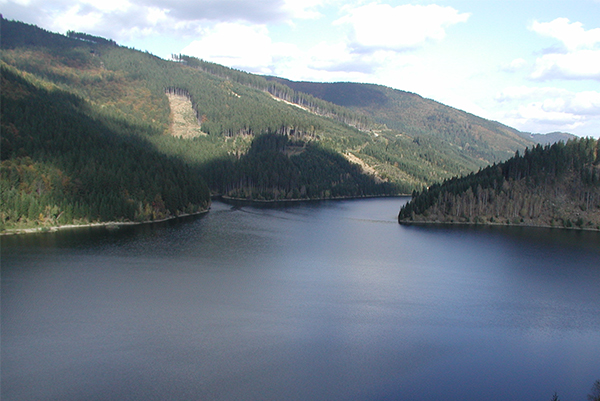
Lake Latte
Foreground Image
Background Image
Naive Copy and Paste
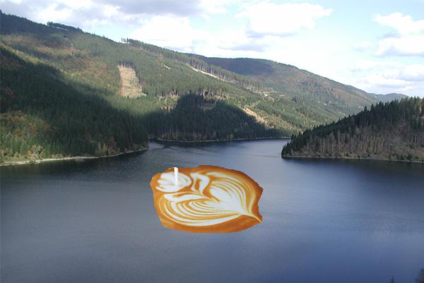
Blending result
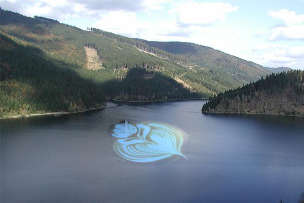
Failure case. The edge blending is pretty bad and the color contrast in the source image w.r.t
the target image means there are some lingering elements of the original brown of the coffee.
Bear Tiger comparison of Multiresoltuion and Poisson Blending
Foreground Image
Background Image
Naive Copy and Paste
Multiresolution
Poisson