Images are basically matrices of intensity values, where you can think of each pixel value as a dimension for the linear basis that determines what the picture looks like. There are other representations for an image basis, and in this project we will explore both the frequency domain and the gradient domain in order to exploit special properties and perform various image manipulation techniques.

Part 1: Frequency Domain

1.1: Image Sharpening

In this part we perform a simple sharpening of an image. Consider an image I. Applying a Gaussian (low pass) filter on the image we get G, and thus I - G gives us the details in the original image. By adding a portion of this back to I, we get a sharpened image.

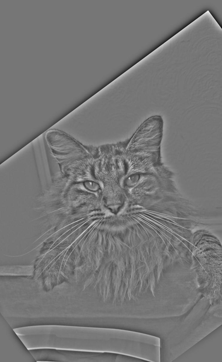
1.2: Hybrid Images

In this section we create hybrid images by combining the high frequency information of one image with the low frequency information of another image. This gives the effect that when looked at closely, you can see the higher frequency details much more clearly. But when looking from afar, your vision can only discern the broader structure of the lower frequency image, thus seemingly shifting that image into view.

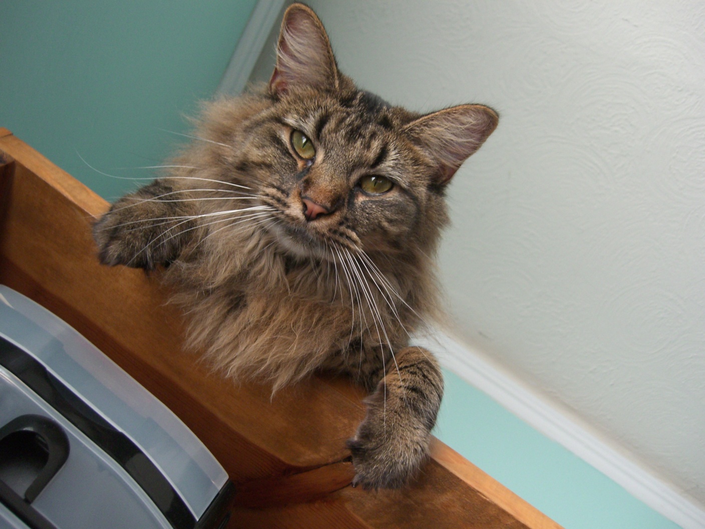
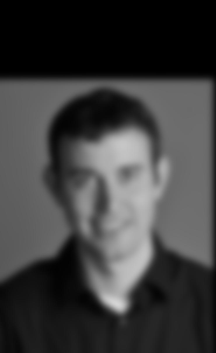
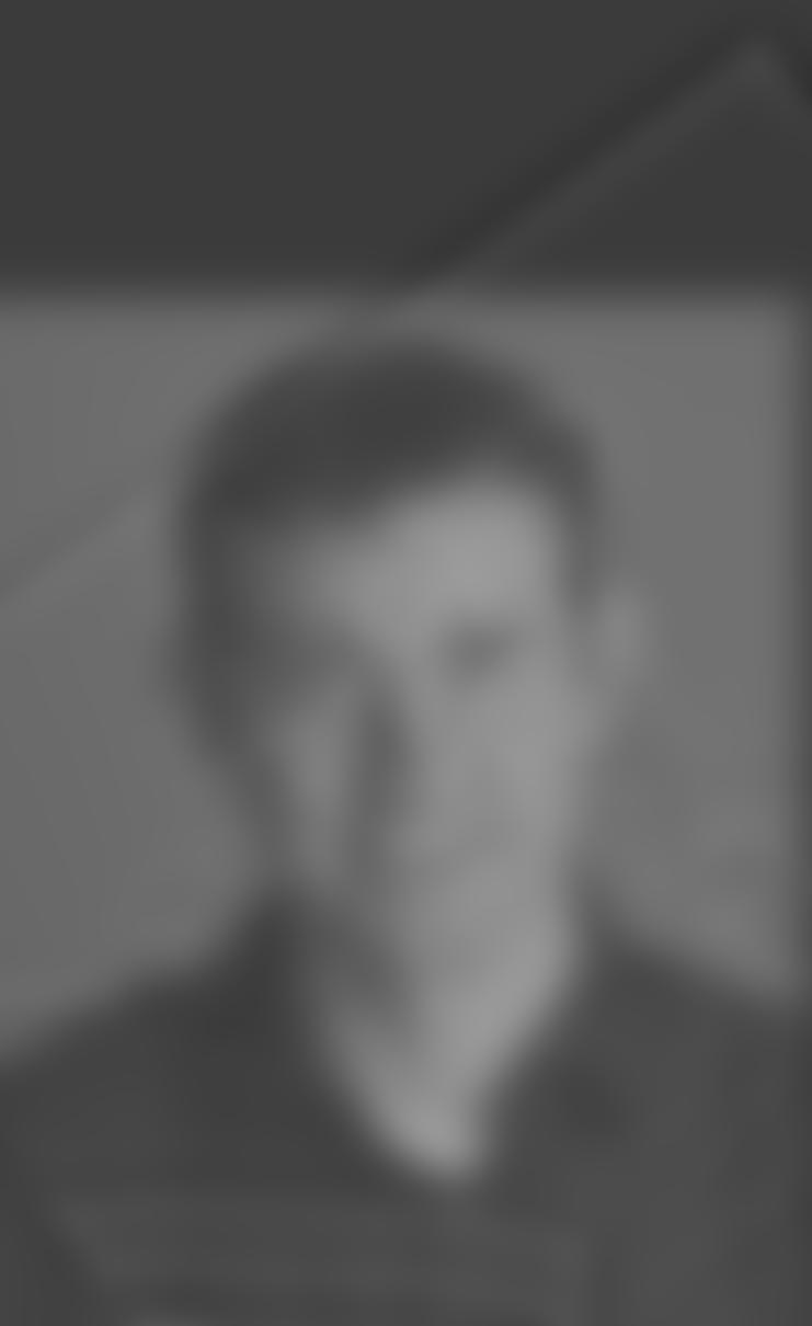
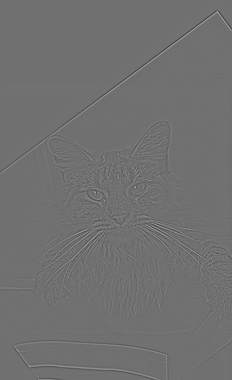
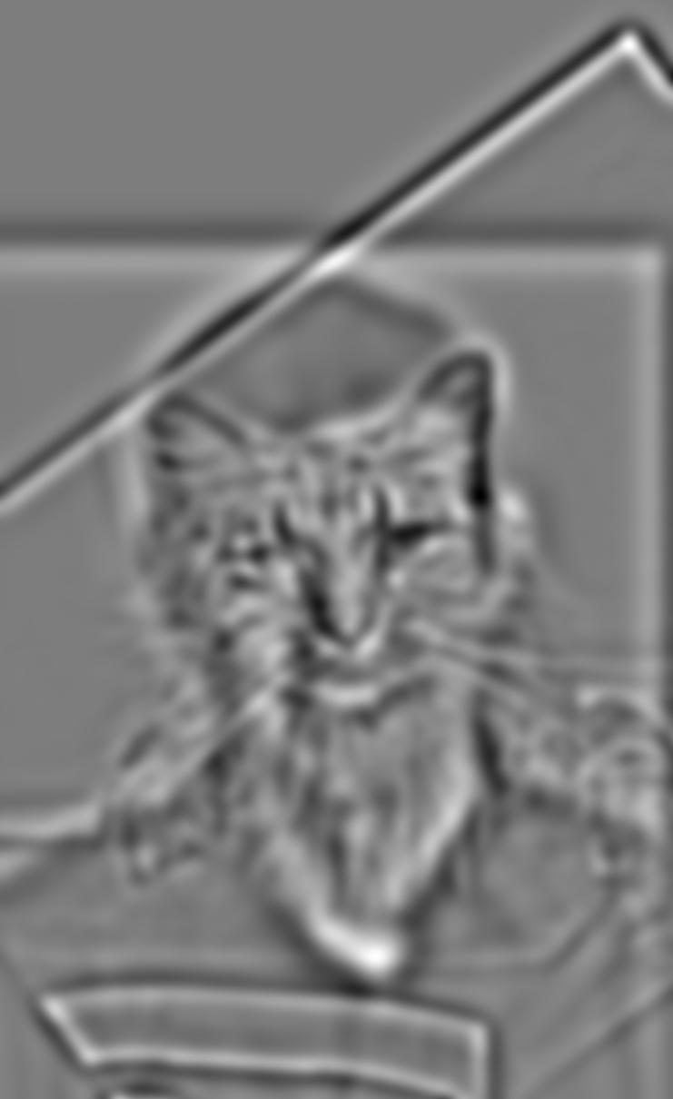
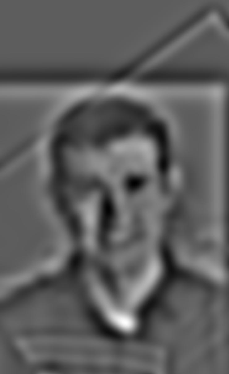
Here we combine Derek (low frequencies) and Nutmeg (high frequencies) the cat.

Fourier Domain Analysis

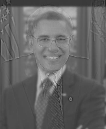
Next we will take a look at the Fourier domain for each of the hybrid halves and then the combined result. The two halves that were averaged together to create the hybrid image are shown below.

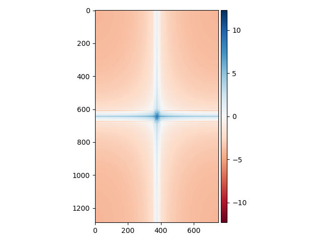
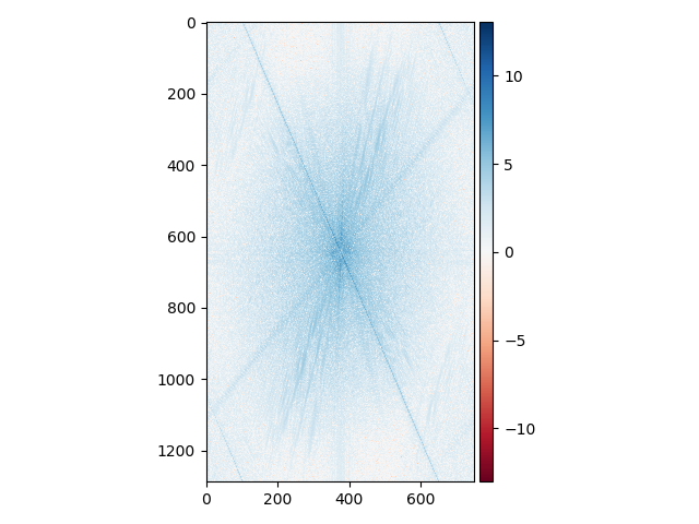
In the first Fourier domain, we see very high intensity values at the very center of the image and along the two axes with radial symmetry. The center will always "on" since we will always have some degree of base intensity for the image (otherwise, it will be all black). The blue axes represent the edges of the blurred image created by the portrait frame, which you can see line up perpendicularly as do the axes in the Fourier image.

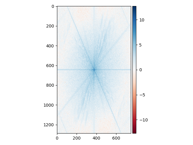
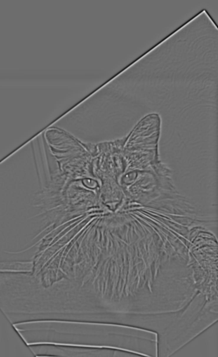
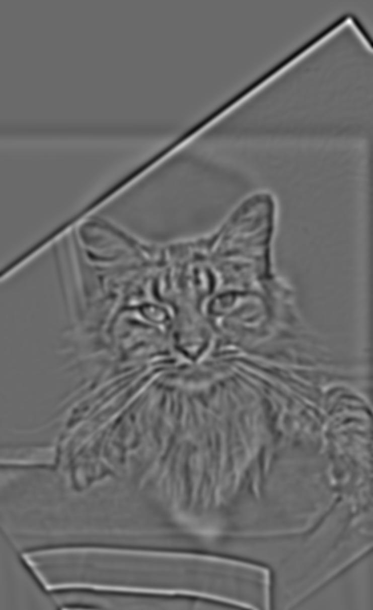
In the middle, the picture of Nutmeg is put through a high pass filter, removing all the lower frequency information. This is why you can see that compared to the next Fourier image, the very center region of this one is less blue, corresponding to zero values in the Fourier basis. There are clear diagonal lines across this image with high values, which represent the edges that had to be represented in the picture due to the rotation during alignment. Several other lighter diagonal streaks towards the middle of the picture probably correspond to Nutmeg's whiskers, which are also fairly long and straight.

In the hybrid image, we see that the very center of the image is definitely more blue than in the middle Fourier image, which means that the low frequency information was added back from blending with Derek. Additionally, because of Derek's portrait frame, we once again have the perpendicular blue horizonal and vertical axes.

Failed examples

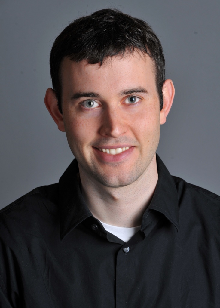
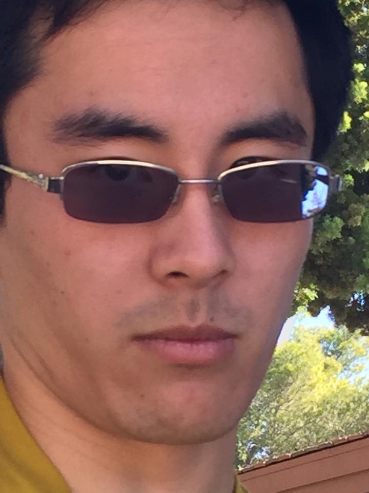
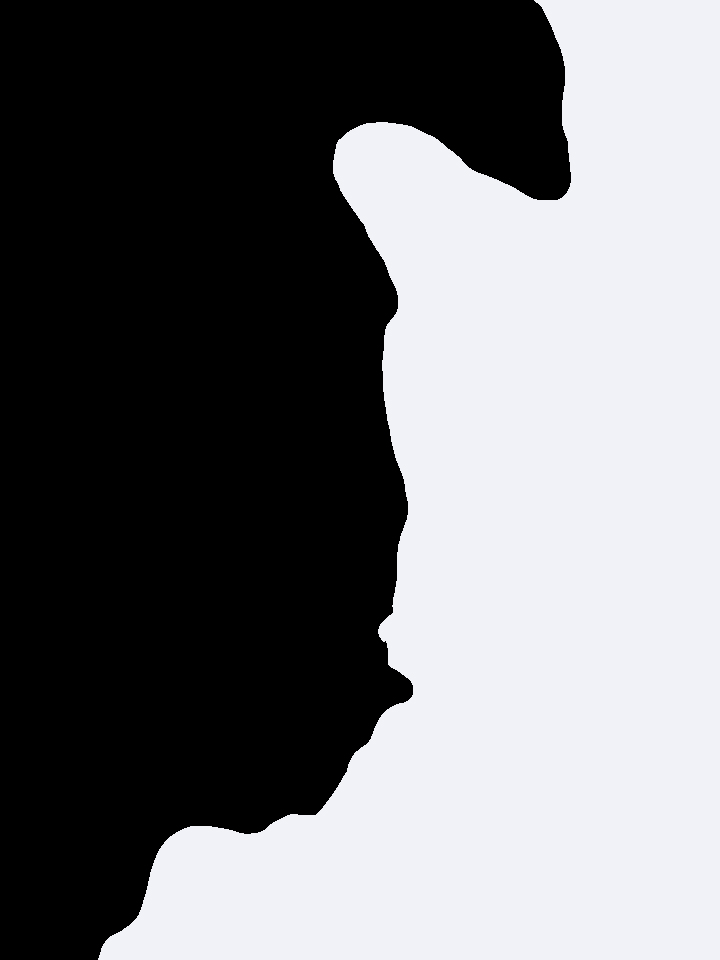
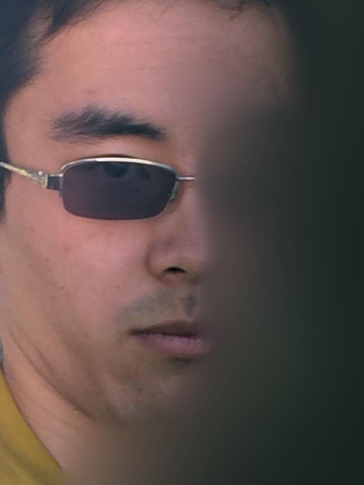
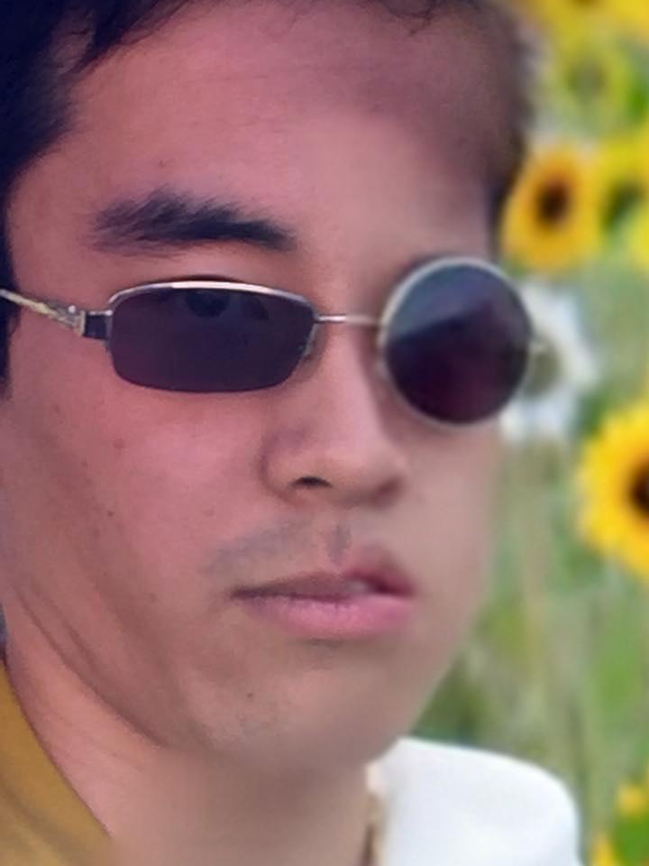
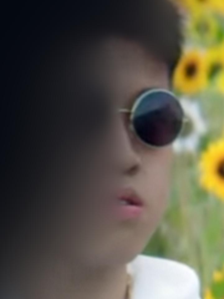
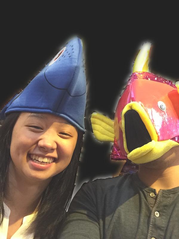
Here's an example that did not turn out entirely as expected. Some people think that I look like a koala, so I created a hybrid image to check it out:

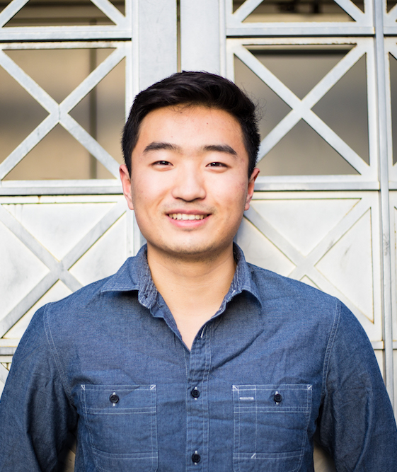
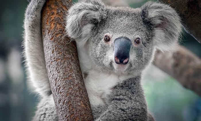
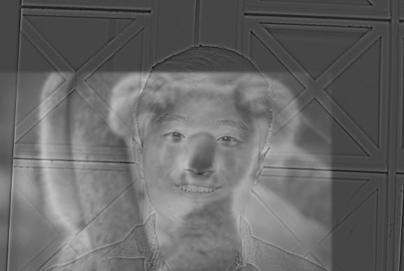
I think they're wrong. My face is much smaller, so the two frames do not mesh up well.

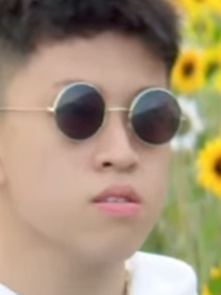
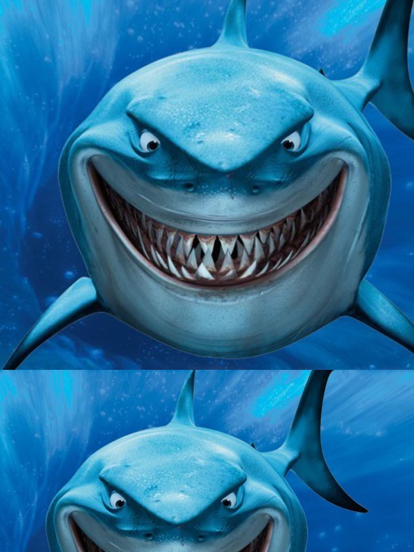
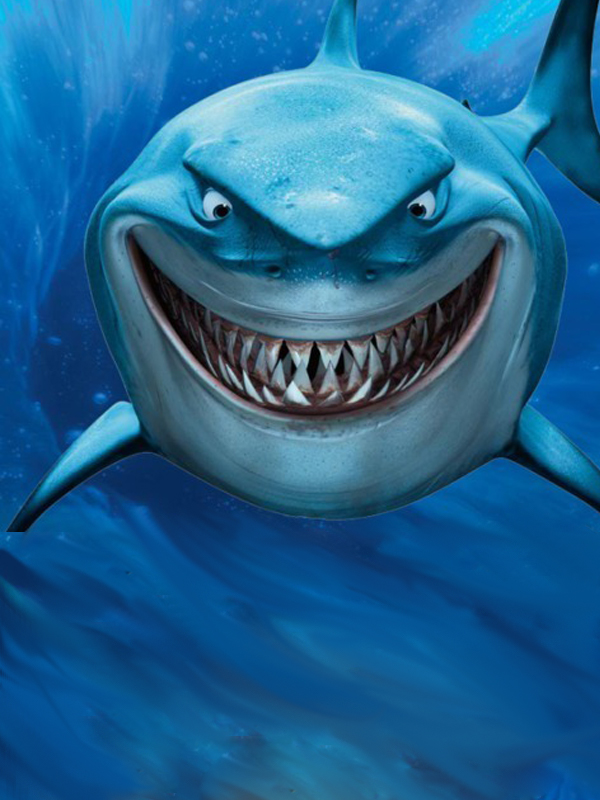
Another example:

1.3: Gaussian and Laplacian Stacks

In this section we prepare tools that will be useful for the next manipulation (multiresolution blending). In particular, we construct Gaussian stacks and Laplacian stacks for storing the frequency slices of images in order to manipulate them separately.

Each image in the Gaussian stack has the same dimensions (not a pyramid), and at each level we exponentially increase the sigma value of the Gaussian kernel. The depth and base/exponent values can be controlled to achieve the desired effect.

The images in the Laplacian stack are constructed by calculating differences between consecutive images in the Gaussian stack. For example, L0, which is the first level Laplacian, is calculated by IMAGE - G0. Similarly, L1 = G0 - G1, and so on.

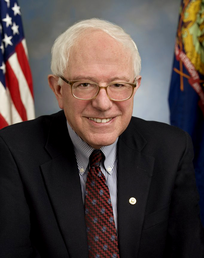
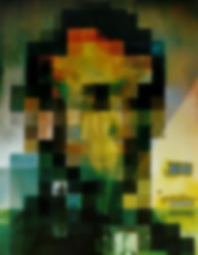
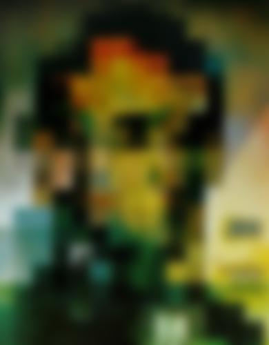
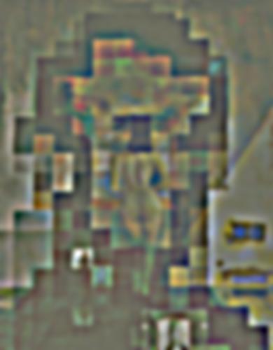
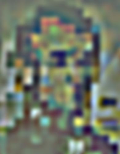
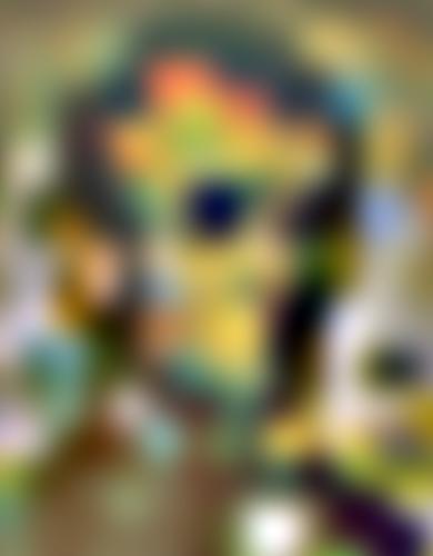
Let's take a look at the same stacks for the Lincoln Gala image.

1.4: Multiresolution Blending

Next we will explore a blending technique which utilizes the Laplacian stacks we just created to perform a hybrid blend. The concept is that higher level Laplacians capture higher frequency "slices" of the image information, so blending them too much would create too many overlapping artifacts. Lower level Laplacians (deeper) are much lower frequency, so they can be overlapped more to create a more even blending composition.

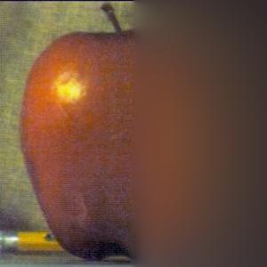
First, let's try to blend and apple and an orange as described in the paper.

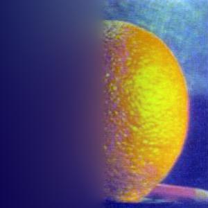
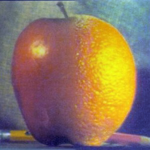
Here are some other ones I tried!

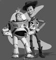
My two good friends.

Here's one that didn't work out too well due to the fact that the mask edge was right along a hard boundary of the image with very different color channels between the images. I had to make sigma much smaller for this and use half the number of layers in the L and G stacks, but the result can still be better.

First I had to use Photoshop to artificially create more vertical space in my image because the orientation didn't match :(

Then we proceed with blending.

Part 2: Gradient Domain and Poisson Blending

In this part of the project, we will use the gradient domain to manipulate images. In particular, we will allow one region of an image to be transported into another image, primarily preserving the gradients between pixels of the original image rather than their pure intensities. This will allow the new pixels transferred to take on the relative color profile of the surrounding target image.

Here is an example:

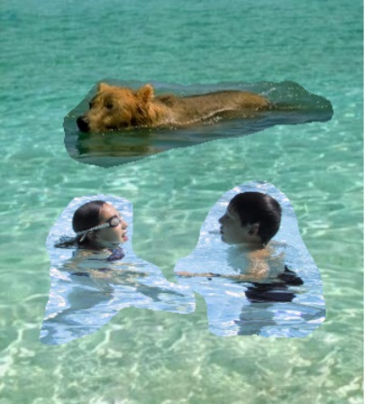
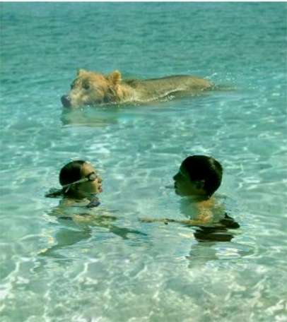
The basic concept is that if we move the region S to the target image T, we will preserve the relative differences in intensities between pixels (specifically we will compute the gradient between one pixel and its four adjacent neighbors in each color channel). The pixels may totally change color, but the shape and form should still maintain its original resemblance.

Another concept is that the newly computed pixels v_i have a similar color profile to the target image due to the boundary conditions, which will be described in the following equation.

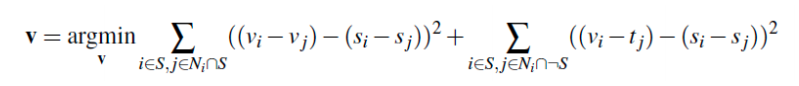
In the first summation we compute a least squares difference between two adjacent pixels in source region S and the corresponding two adjacent (computed) pixels that we will place into T. The difference should be minimized, which is what this part says.

The next part describes the boundary condition and is what will determine the overall color profile of the newly computed region. Basically when we are looking at a source pixel's neighbor that does NOT belong in the region S, then we only need to compute the single pixel v_i in the target image T based on its difference to the adjacent pixel in T.

We will solve for all v_i's simultaneously using a linear system and a sparse matrix A. For each pixel in the source image, we provide a new linear constraint, and thus we add a row to our matrix and a corresponding element in vector b. Because our resulting matrix is square, we can use a sparse matrix solver to get the solution vector x, which is the linearized form of the pixels that we need to insert to the target image. I used a least squares solver as well, but that ended up taking way too long to converge, maybe 5-10x as long as the sparse matrix solver.

2.1: Toy Problem

In this part we take a slightly different approach to the Poisson blending problem. Instead of transporting just a region of pixels from one image to another, we will attempt to reconstruct the entire image. This is equivalent to transposing all pixels.

We establish x and y directional derivatives and try to preserve the differences as much as possible as described above. In addition, since there are no pixels beyond the boundary (which is the entire image), we have to add a final constraint that the left top pixel has to be equal in our solution.

2.2: Poisson Blending

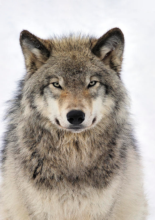
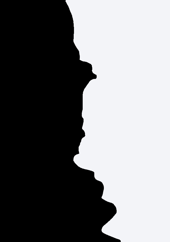
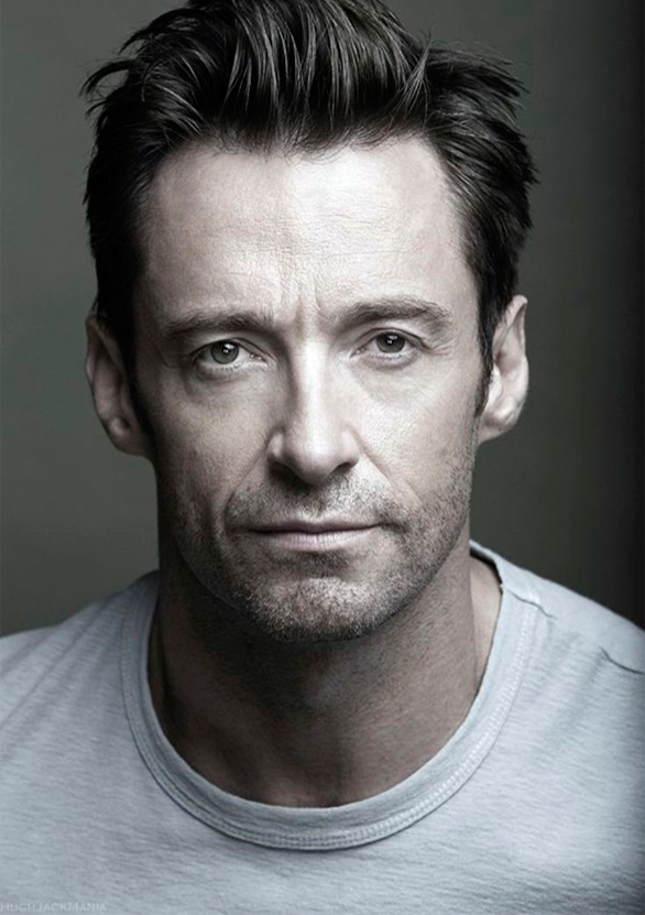
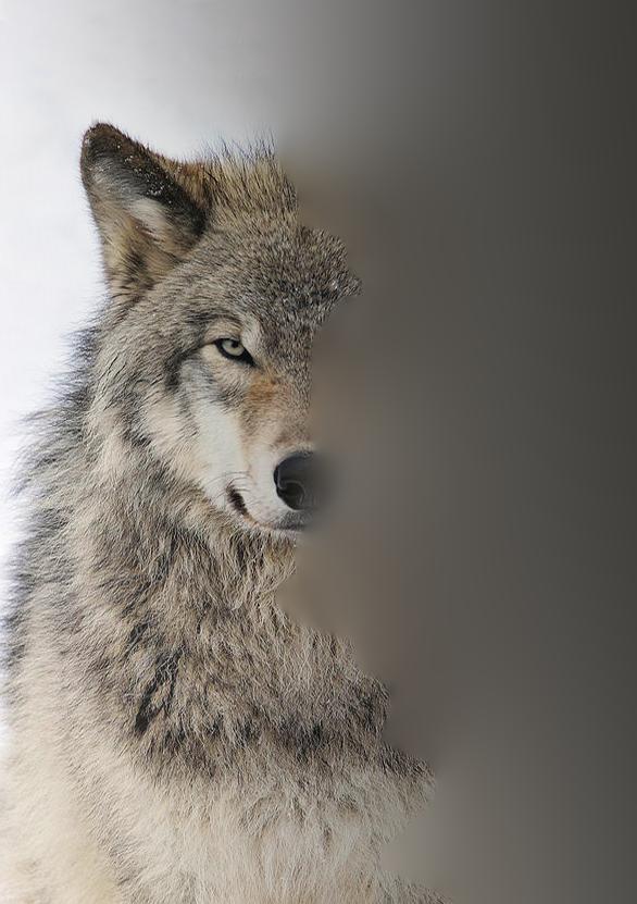
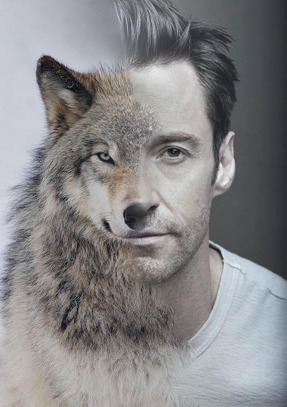
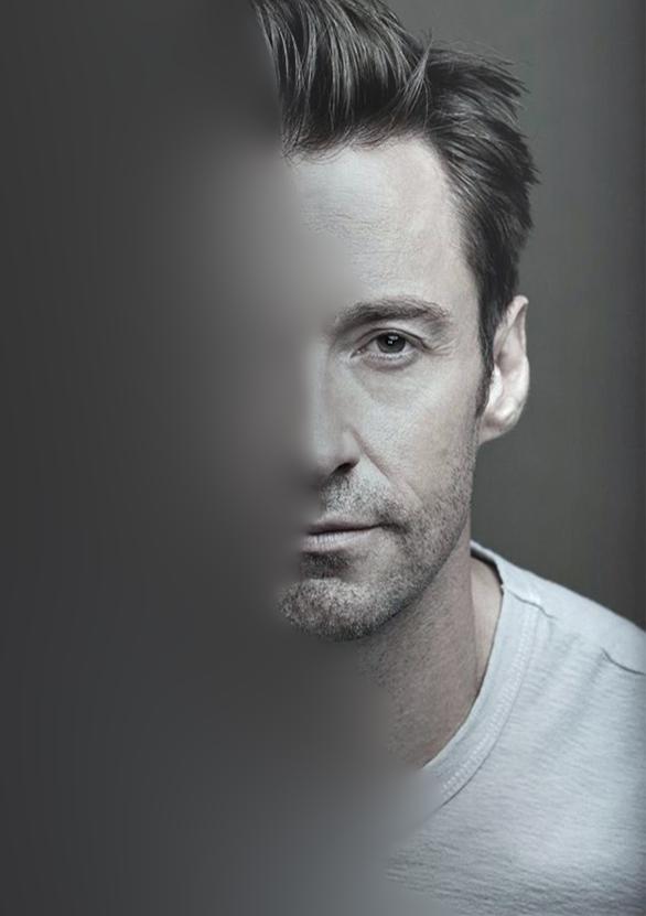
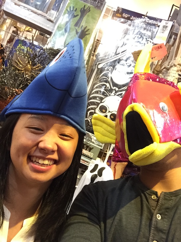
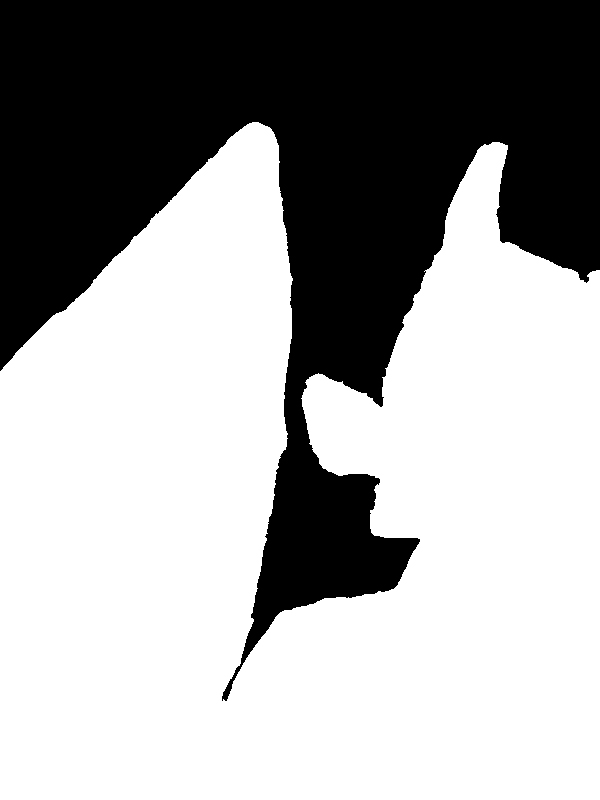
With the Poisson blending procedure detailed above, I took a look at what differences the technique would provide versus the multiresolution blending we used earlier. Here is Hugh Jackman and the wolf again.

This technique is pretty slow on my computer, since we have a matrix with many millions of entires. Thus, I will downscale the images to 30% the original.

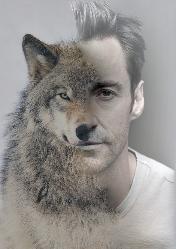
Evidently, there are some issues with Poisson blending here, as the mask I used incorporated way too large of a region for the algorithm to properly interpret the pixel intensities that are far away from the border. Thus, everything on the right, which was computed, is desaturated by the tints of uniform colors from the left source.

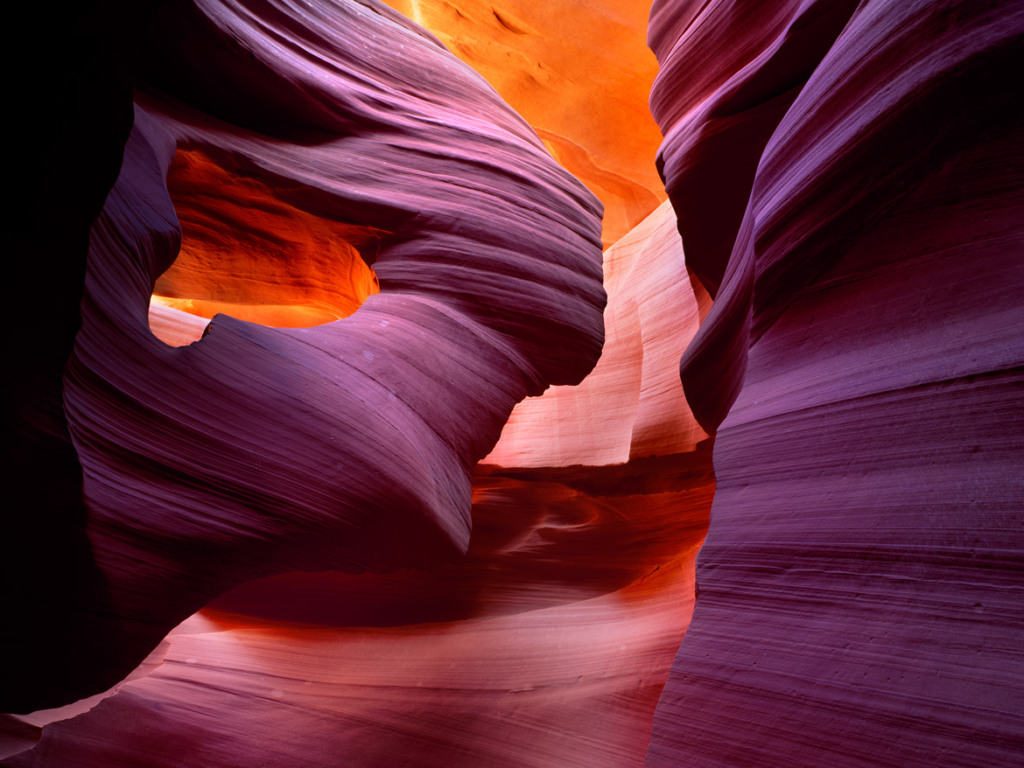
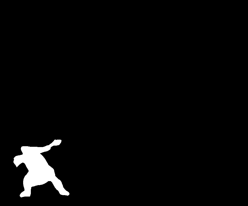
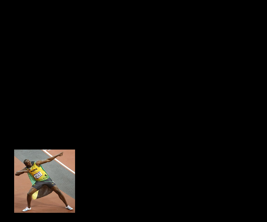
I hypothesized that Poisson blending would be much more effective if the masking region were much smaller and fully contained (not along the border of the image, where it can't extract color information from adjacent pixels). Another feature that would help improve the results is to find a region on the target image with minimal or at least uniform gradient differences (think an ocean or desert) and also capture source pixels with minimal gradients that surround the object intended to be transposed. In the end, I found a picture of Usain bolt with his classic pose and transposed him into an apocalyptic environment.

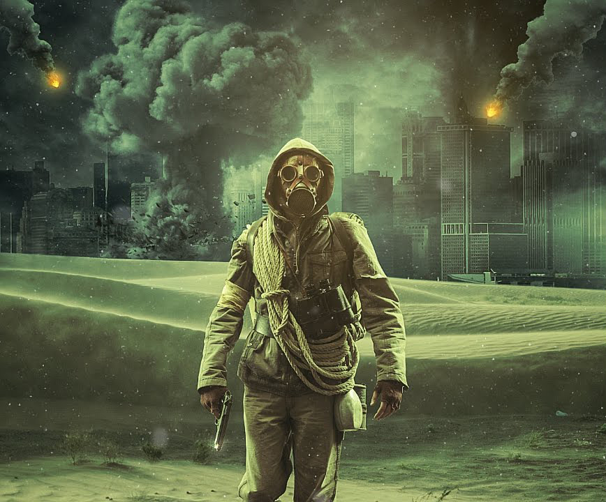
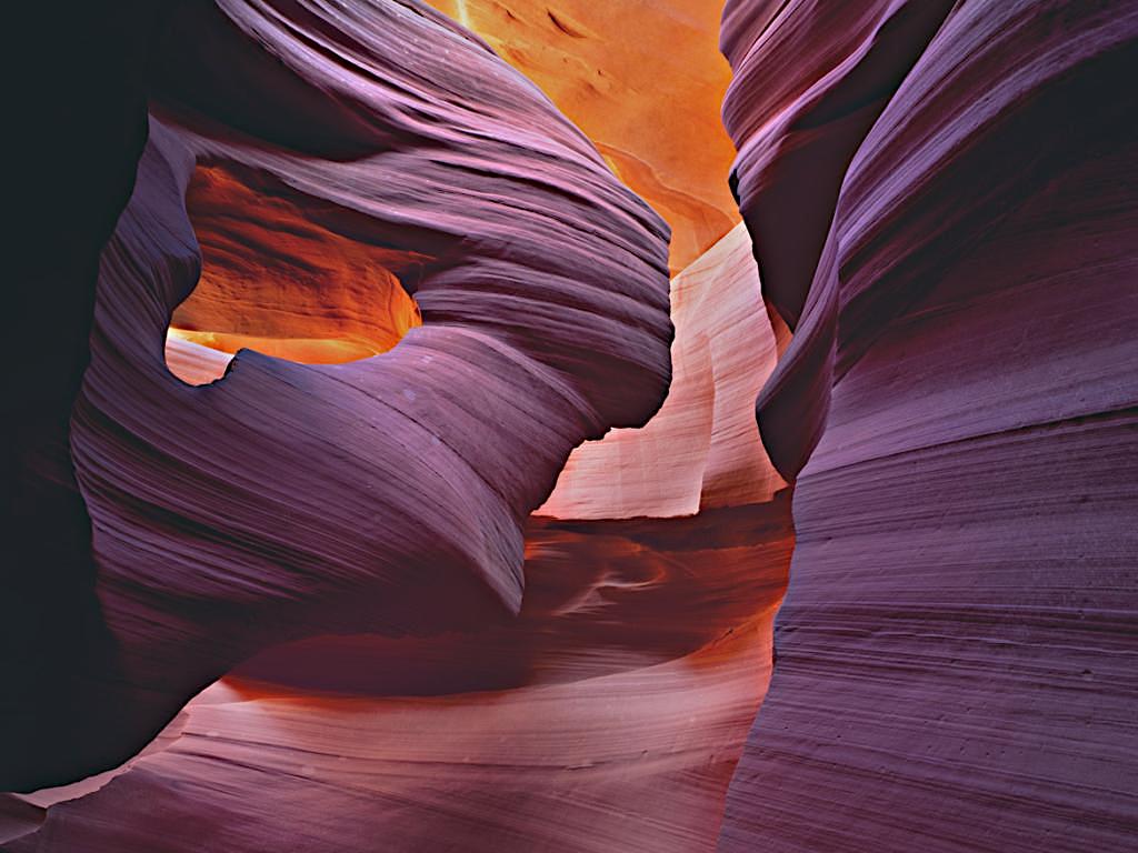
The initial result left some room for improvement, and I noticed that the image was significantly desaturated compared to the original. I realized that it was actually due to the final normalization that I apply to the whole image. Usain's skin color is actually much darker than the pixels from the apocalypse image, so by normalizing the picture with him inside it desaturated everything else.

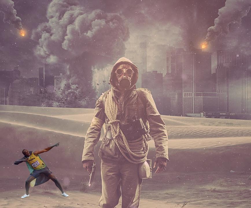
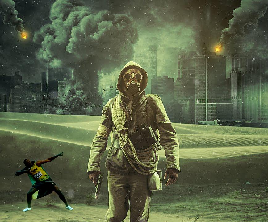
I had to come up with a "mask normalization" function, which basically did the normalization to the final image using intensity values of only the pixels excluded by the mask (everything except Usain). This gave a much better result

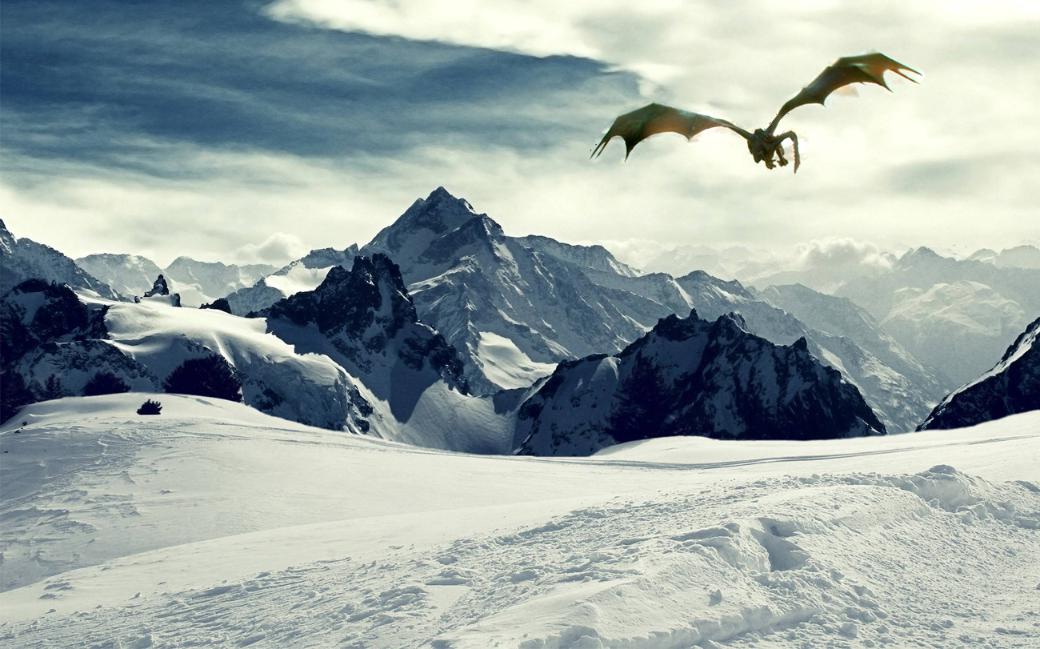
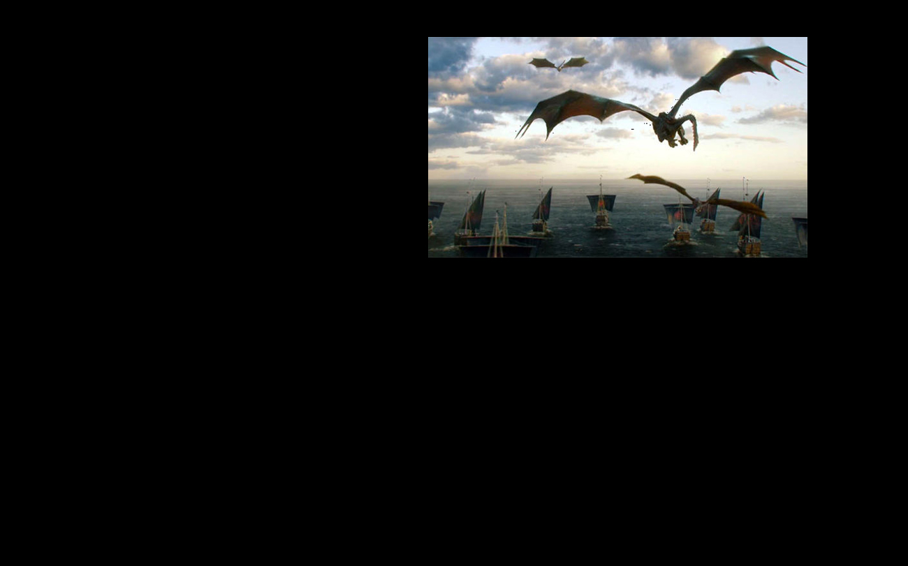
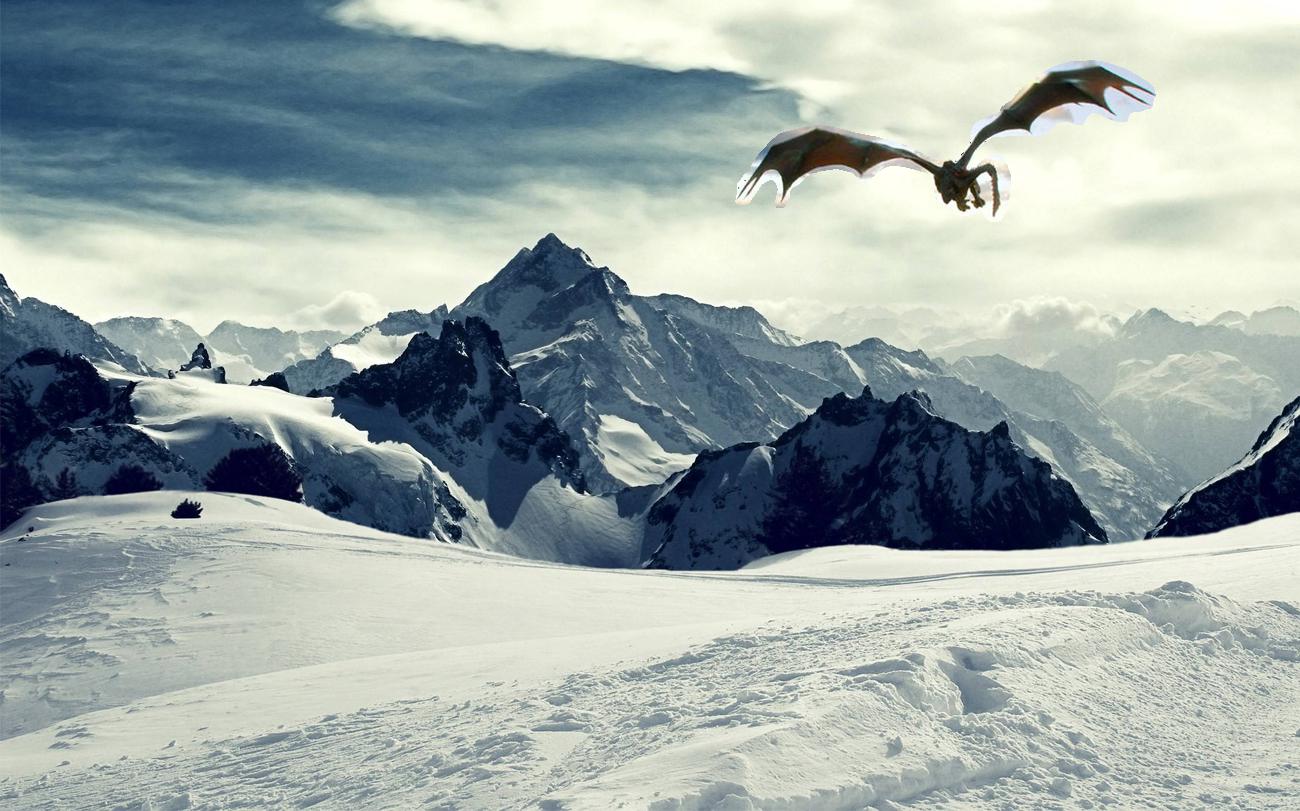
For a final example I copied Viserion into the sky overlooking a nice snowy mountain.

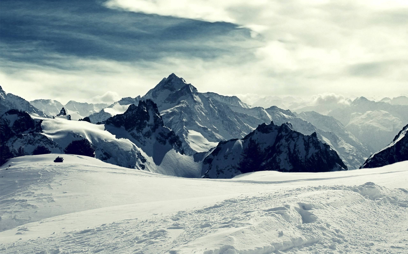
Here are the individual color channels just for fun:

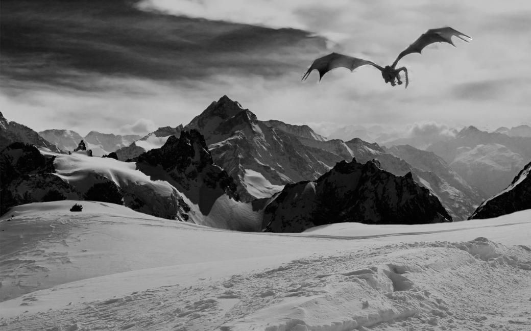
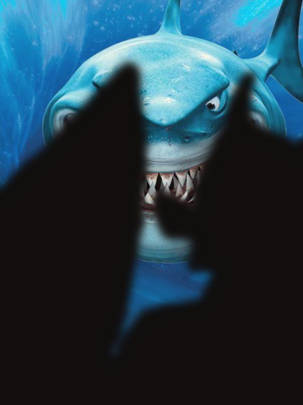
If we had just copied the pixels it would look like this, with a defined edge and color differences:

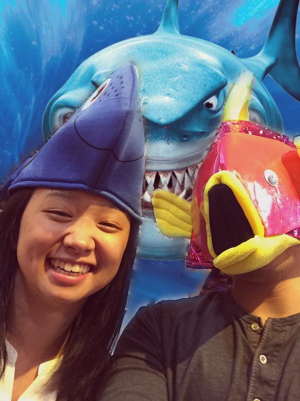
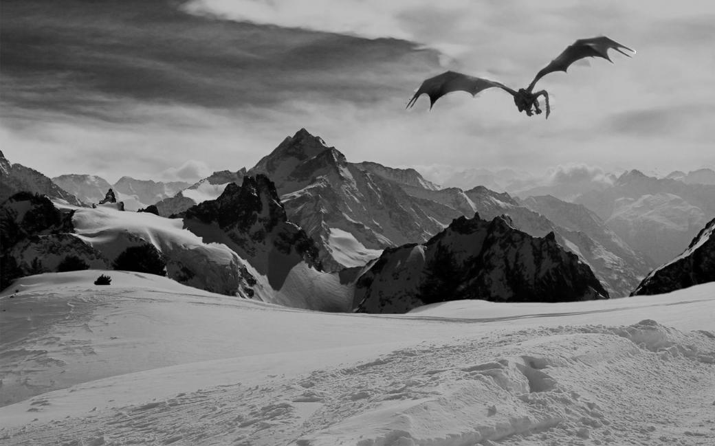
But blended properly gives the final result: