Fun with frequencies
Zhen Qin
1.1 Warm-up
In this part, we use a gaussian filter to blur the original picture. Subtract the alpha, a constant between 0 and 1, times the blurred image from original image, we get the sharpened image. Then we add the sharpened image to the original image to get the sharpened effect.
In conclusion, the math is:
Output = (1 + alpha*image) + alpha*gaussian_convoluted_image
Following of is the output with gaussian filters with different sigma and alpha value, we can see that bigger sigma (variance) gives us wider edges in sharpened output and bigger alpha gives more sharpened images:

Origin Image

Sigma = 1
Alpha = 1

Sigma = 1
Alpha = 2

Sigma = 1
Alpha = 5

Sigma = 2
Alpha = 1

Sigma = 2
Alpha = 2

Sigma = 2
Alpha = 5
Sigma = 5
Alpha = 1

Sigma = 5
Alpha = 2
Sigma = 5
Alpha = 5
1.2: Hybrid Images
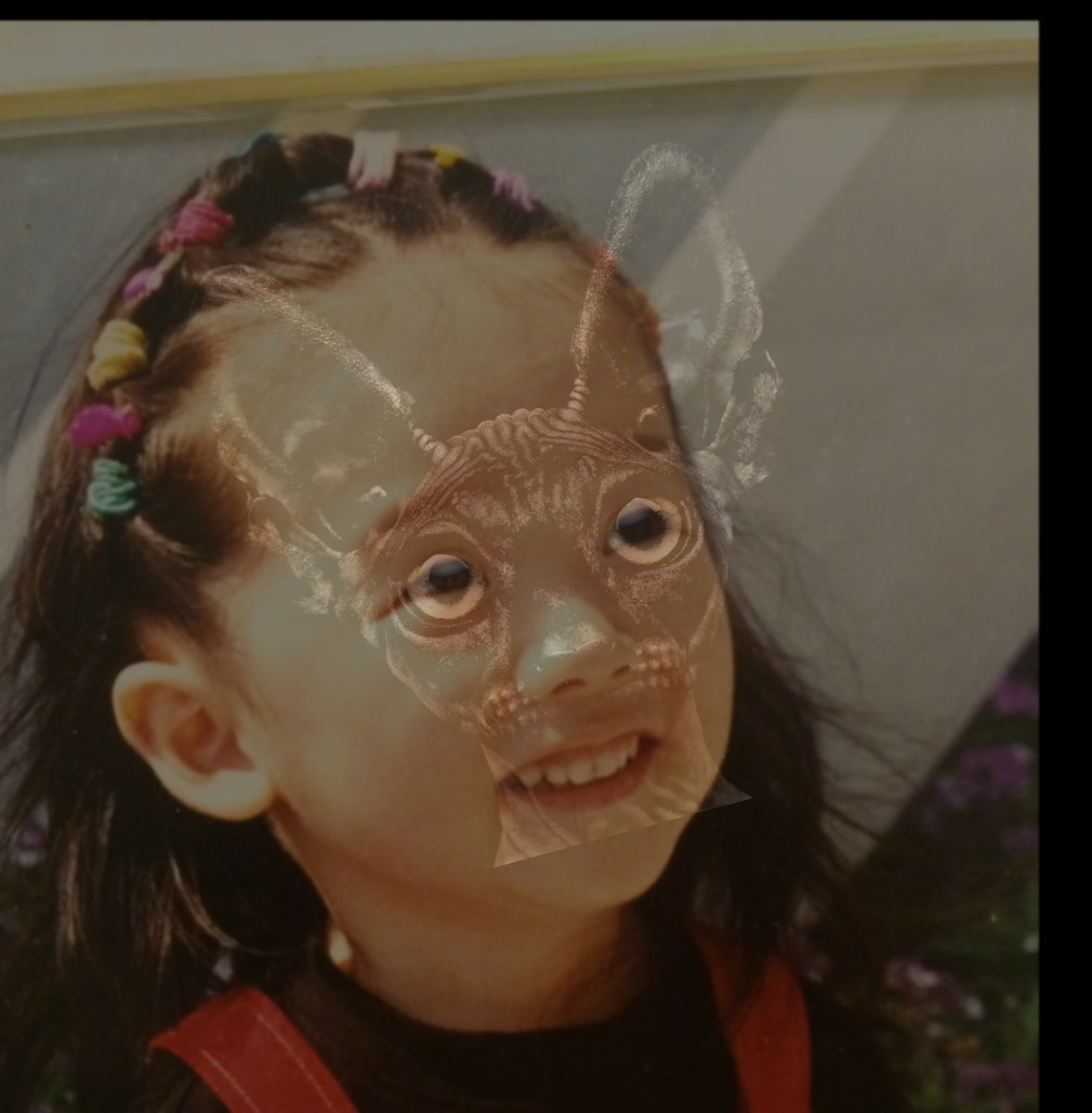
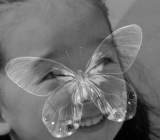
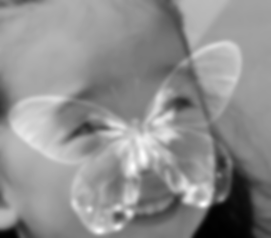
To combine two images, we can perform low-pass filtering on one, and high-pass filtering the other one. I use Gaussian filter as the low pass filter, and laplacian filter as high pass filter. In the end simply add the two filtered images into a single hybrid image. The low-pass filtered image retains mostly low frequencies, while the high-pass filtered one contains mostly high frequencies. At close distances, the human perceptual system can detect and make sense of the high frequencies present in the image. When we move further away, we can only really see the lower frequencies. Therefore, with these hybrid images, we can see two different images depending on how close we are to the image when viewing it.
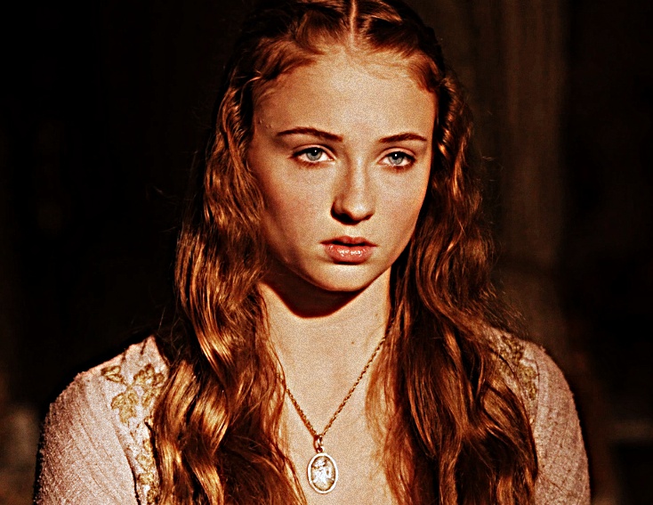
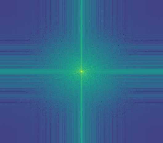
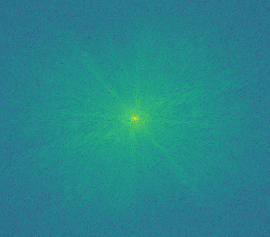
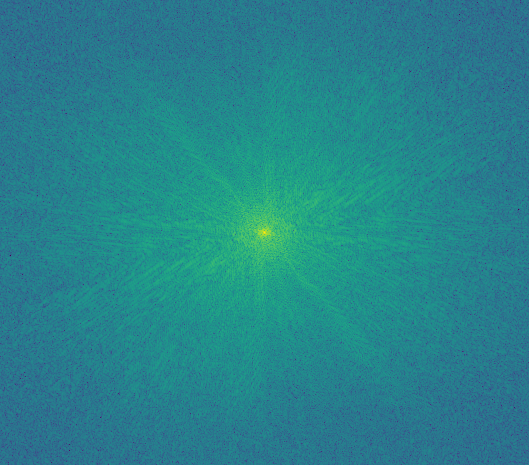
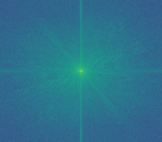
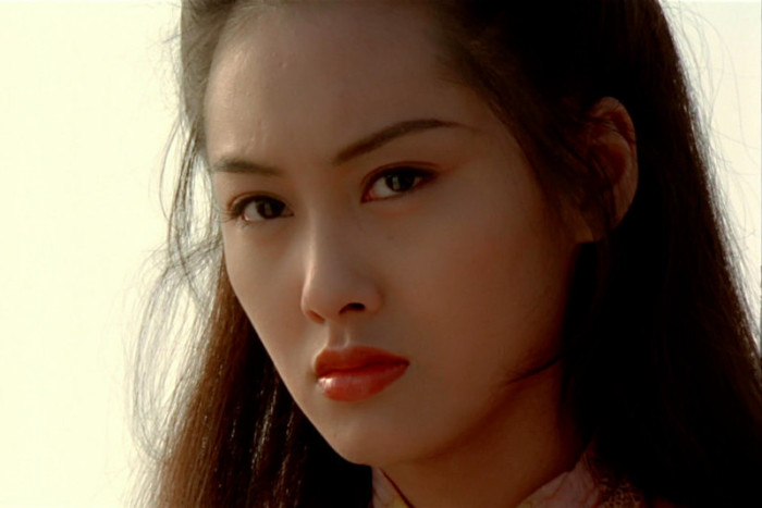
The following is my favorite result with the Fourier transform of the image shown. The girl is low pass filtered, and the butterfly is high pass filtered. After combing the two images, we get a magical mask on the girl’s face. From the Fourier transform, we can the frequency difference after a low-pass and high pass filtered image.
Girl and butterfly
Input Image Girl

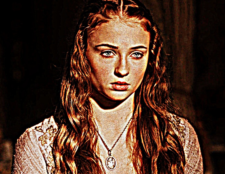
Low pass filtered Image
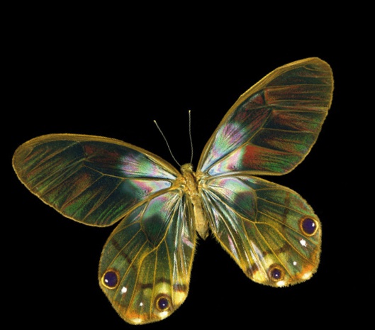
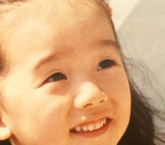
Input Image Butterfly
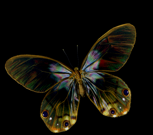
High pass filtered Image
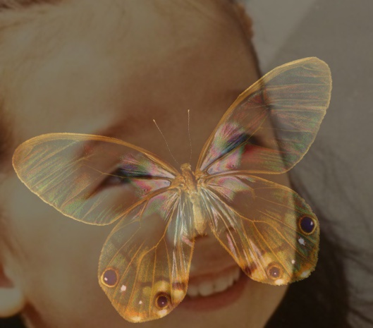
Hybrid Image
FFT analysis for Girl and butterfly
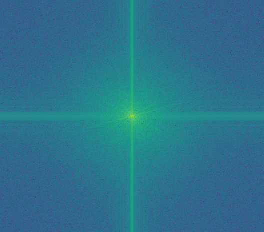
Input Image Girl
Low pass filtered Image
Input Image Butterfly
High pass filtered Image
Hybrid Image
Following one more example that take a girl’s face is high pass filtered and the background sunset is low_pass filtered. The hybrid piture creates a romantic and sorrow feeling when thinking of a past lover.
Past Lover
Input Image for Girl
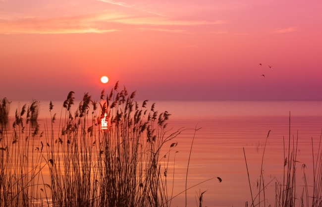
Input Image for sunset
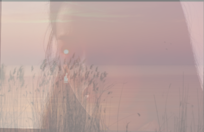
Hybird image
Following is a failed case. This case is failed because the face of the strange cat can’t align with the girl’s face very well.
Failed case
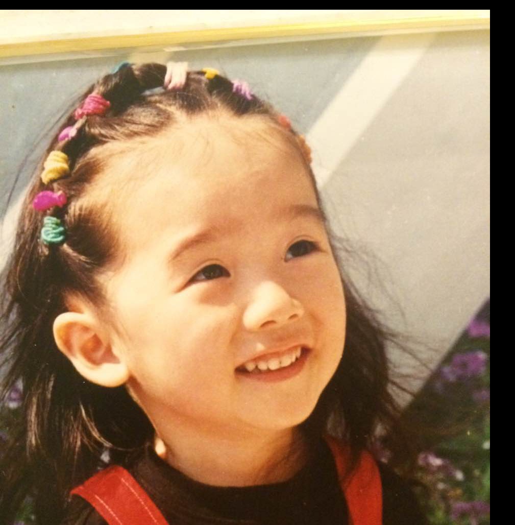
Input Image for Girl
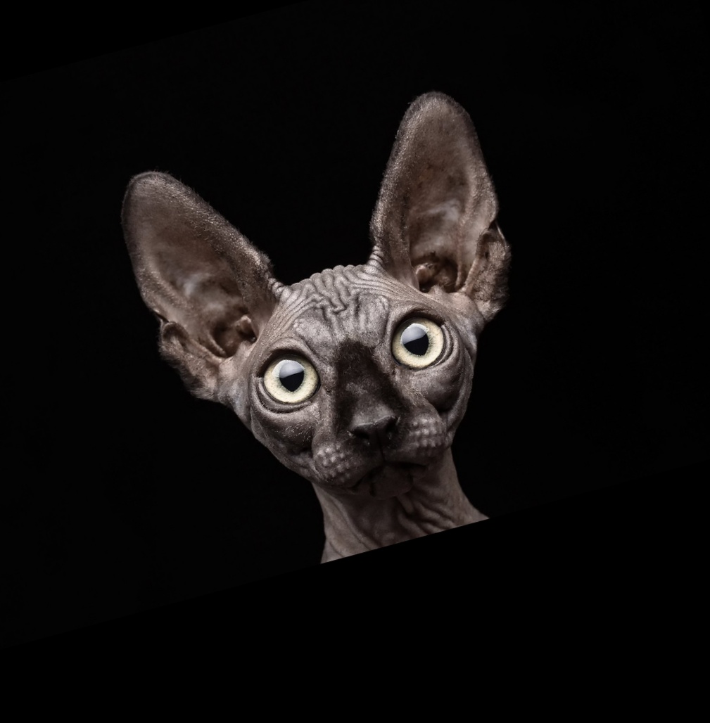
Input Image for strange cat
Failed Hybird image
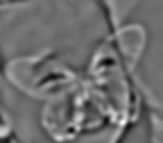
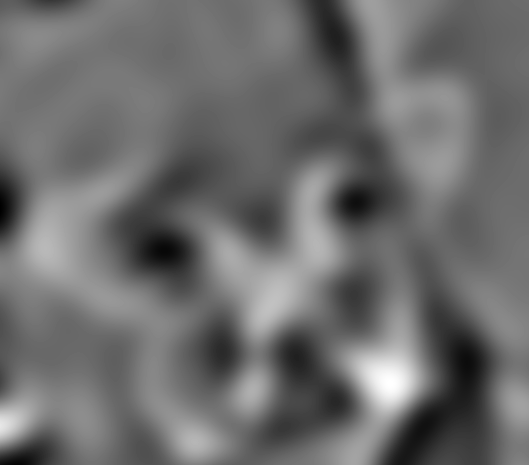
1.3: Gaussian and Laplacian Stacks
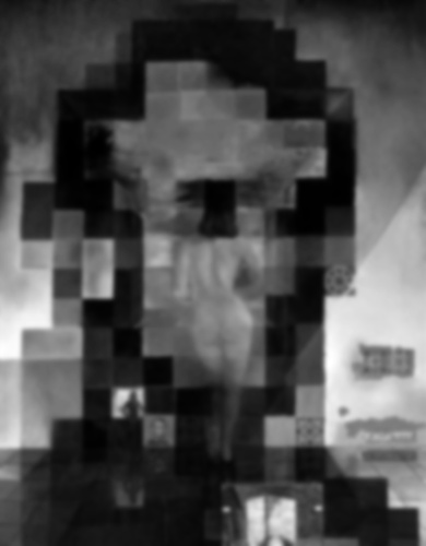
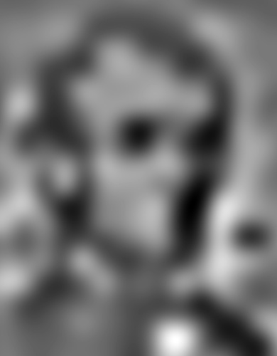
To compute Gaussian and Laplacian stacks, I first first convolute each image with a Gaussian filter of increasing sigma (2, 4, 8, 16, 32). Then at each level I took the difference of the previous and current Gaussian to get the Laplacian. We can find that the high frequency picture dominates when we use small sigma for laplacian filter and the low frequency picture dominates when we use large sigma for gaussian filter. The first level of laplacian filter are all zeros because we simply subtract original picture from itself at this level.
Gaussian filtered of Lincoln:

Sigma = 1
Sigma = 2

Sigma = 4
Sigma = 8

Sigma = 16
Sigma = 32
Laplacian filtered of Lincoln:

Sigma = 1
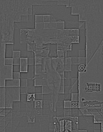
Sigma = 2

Sigma = 4
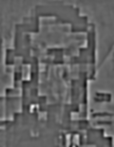
Sigma = 8
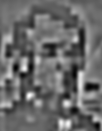
Sigma = 16
Sigma = 32
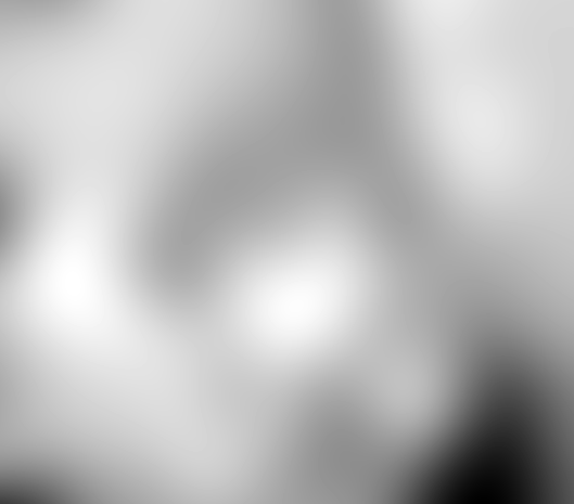
Gaussian filtered of Girl and butterfly from Part1.2:
Sigma = 1

Sigma = 2
Sigma = 4
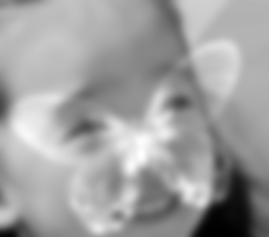
Sigma = 8
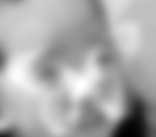
Sigma = 16
Sigma = 32
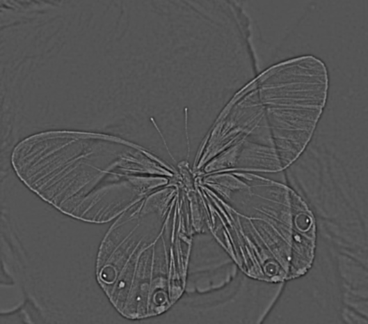
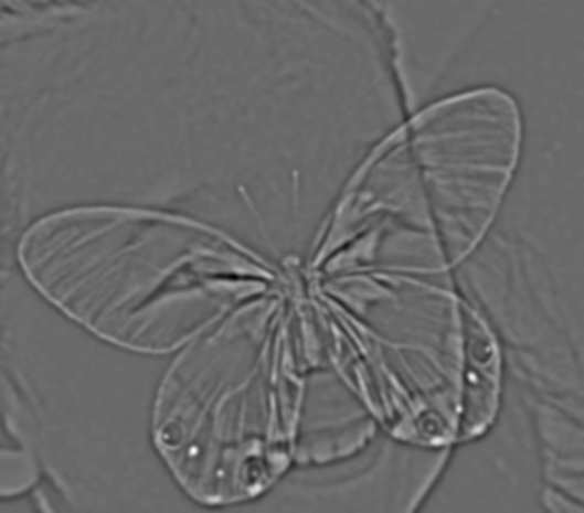
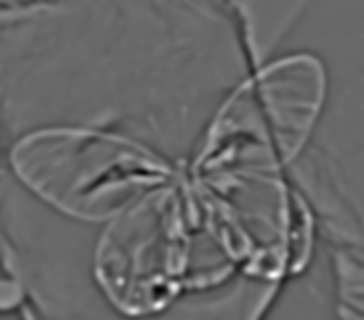
Laplacian filtered of Girl and butterfly from Part1.2:

Sigma = 1
Sigma = 2
Sigma = 4
Sigma = 8
Sigma = 16
Sigma = 32
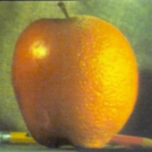
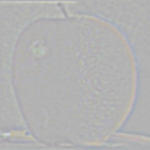
1.4 Multiresolution Blending
In this part I blend two images seamlessly using a multi resolution blending as described in the 1983 paper by Burt and Adelson. An image spline is a smooth seam joining two image together by gently distorting them. Multiresolution blending computes a gentle seam between the two images seperately at each band of image frequencies, resulting in a much smoother seam.
To implement multi resolution blending, I started by taking two images and creating a laplacian stack at each level for both of them. Each laplacian stack is the difference between last level’s gaussian stack and this level’s gaussian stack. In addition, I use the gaussian filter with same sigma to filter the mask as well. Finally, blend both images with the mask at each level and add them together.
The difficulty that I encountered is that at first I forget to add the last level of gaussian stack, so the image is very dark.
Result for apple and orange

Input apple image

Input orange image
Blended Apple and Orange
Blending at each level for apple and orange
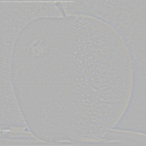
Laplacian stack 0
Laplacian stack 1
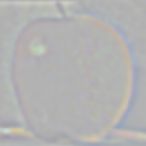
Laplacian stack 2
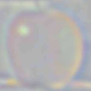
Laplacian stack 3

Laplacian stack 4

Laplacian stack 5

Last gaussian stack
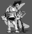
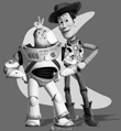
Result for Twillight
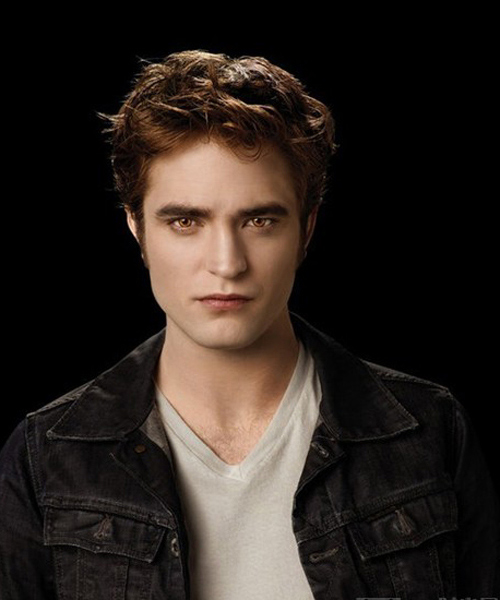
Input Edward image
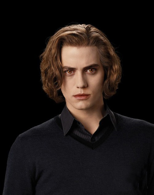
Input Jaspar image
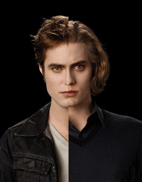
Before Blending

After Blending
Blending at each level for Twillight
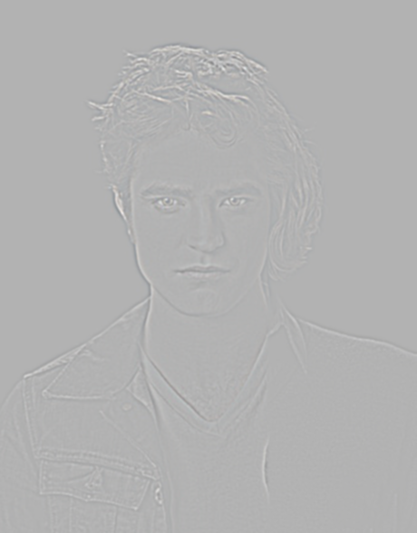
Laplacian stack 0
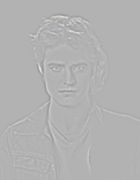
Laplacian stack 1

Laplacian stack 2

Laplacian stack 3

Laplacian stack 4

Laplacian stack 5

Last gaussian stack
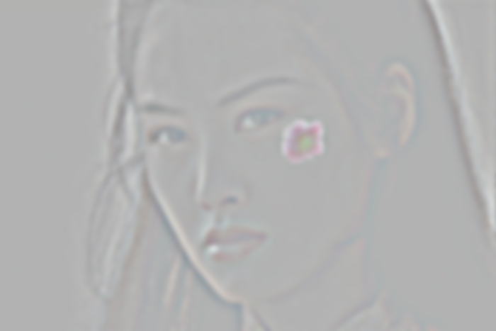
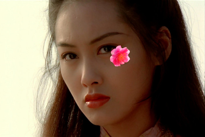
Result for flower on face
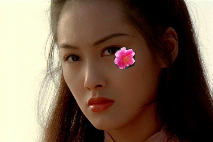
Before Blending
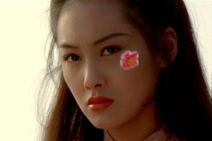
After Blending
Blending at each level for flower on face
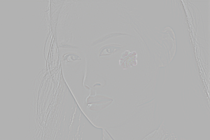
Laplacian stack 0
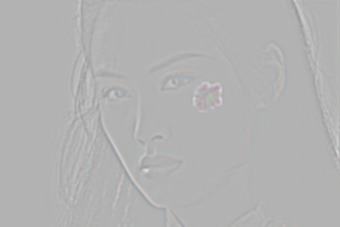
Laplacian stack 1
Laplacian stack 2

Laplacian stack 3

Laplacian stack 4

Laplacian stack 5

Last gaussian stack
Part 2: Gradient Domain Fushion Introduction
This project explores gradient-domain processing, a simple technique with a broad set of applications including blending, tone-mapping, and non-photorealistic rendering. For the core project, we will focus on "Poisson blending"; tone-mapping and NPR can be investigated as bells and whistles.
The primary goal of this assignment is to seamlessly blend an object or texture from a source image into a target image. The insight we will use is that people often care much more about the gradient of an image than the overall intensity. So we can set up the problem as finding values for the target pixels that maximally preserve the gradient of the source region without changing any of the background pixels.
2.1 Toy example
After taking derivative of the L2 Norm, the solution for the least square problem in the is Ax=b. A is the matrix that each column and row represent one pixel from the original matrix. A[i,j] is seated to -1 if jth pixel is a neighbor for it pixel on source image. And all the A[i,i] where ith pixel is outside the mask in the background picture, we set A[i,i] to 1. For all the A[i,i] where ith pixel is in the mask from source picture, we set A[i,i] to its original pixel.In the toy example, the only pixel that is outside the mask is pixel (0,0), and we set that pixel to a fixed value, 0. Through copying the gradient, we recover the image:
Original image
Recovered image
2.2 Poisson Blending
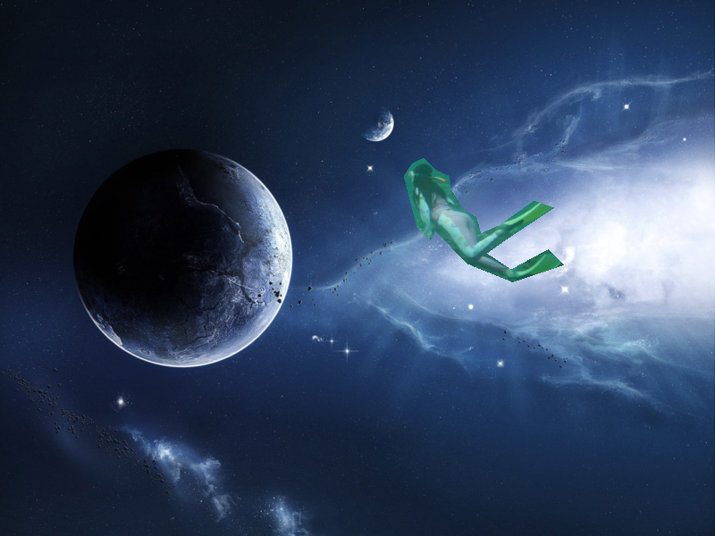
The following is my favorite result from Poisson blending. One of the input image is a picture of myself snorkeling In Palau. I blended this picture with a space. I find out that even the original background of target picture is very green, but after poisson blending, it blends perfectly with the new background.
Swimming in the space
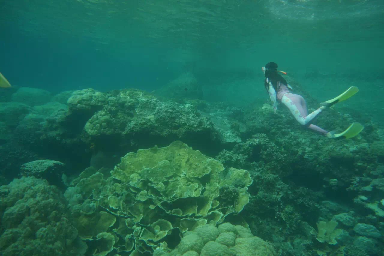
Source
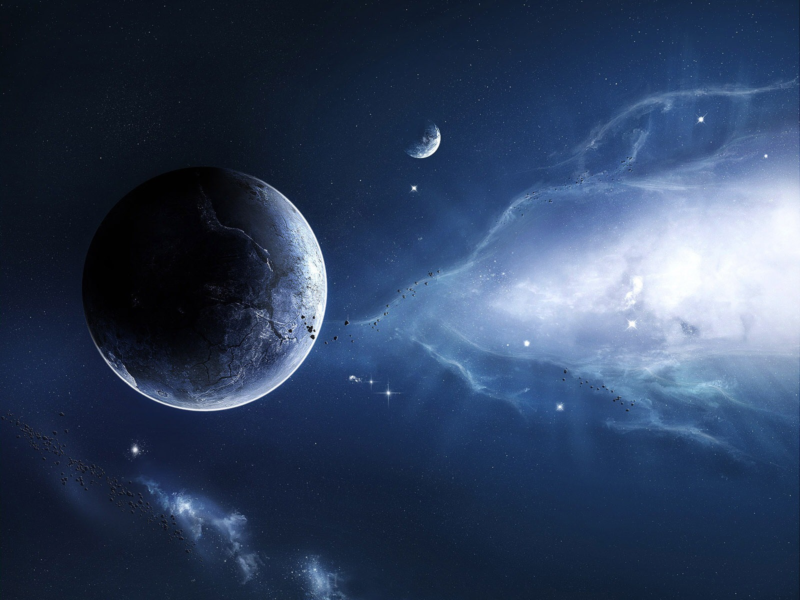
Target
Before Blending

After Blending
Here is one more example: Old town and ship
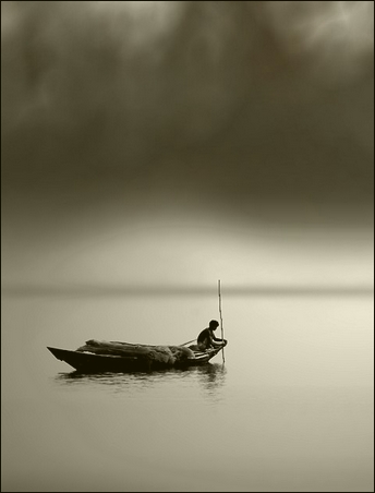
Source
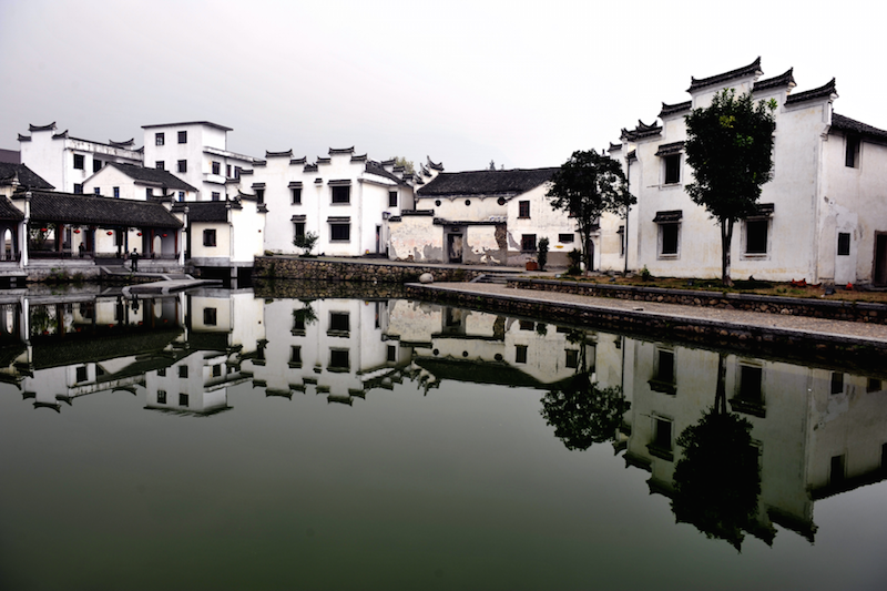
Target
Before Blending
After Blending
Failed example and improvements
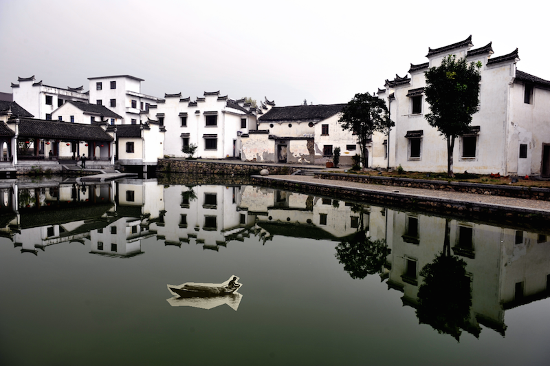
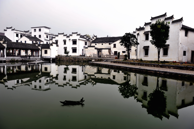
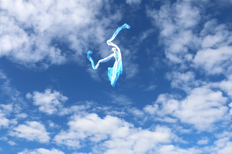
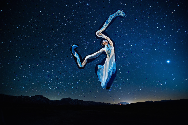
The following is a failed example. Because the original background of the source image, the dancer, is much darker than the dancer itself, and our new background is more bright. Since we are copying over all the gradients. The difference between source images and its original background does mater. The output blended image is too bright and looks natural. Therefore, I changed to use a darker background and the results looks much better:
Failed example: Dancing in the sky
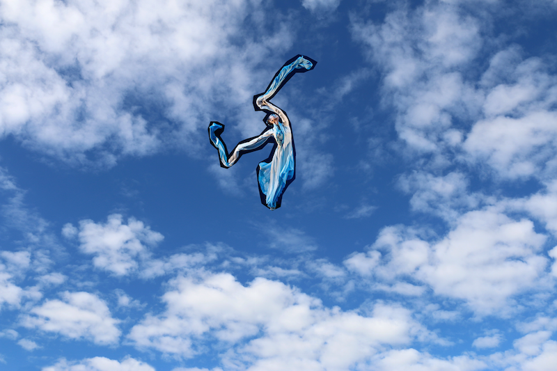
Failed example: Before Blending
Failed example: After Blending
Success Example: Dancing in the sky
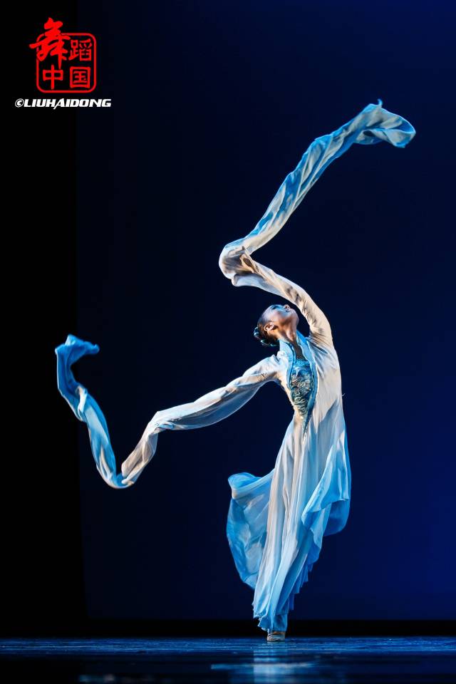
Source
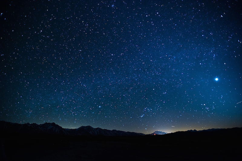
Target
Before Blending
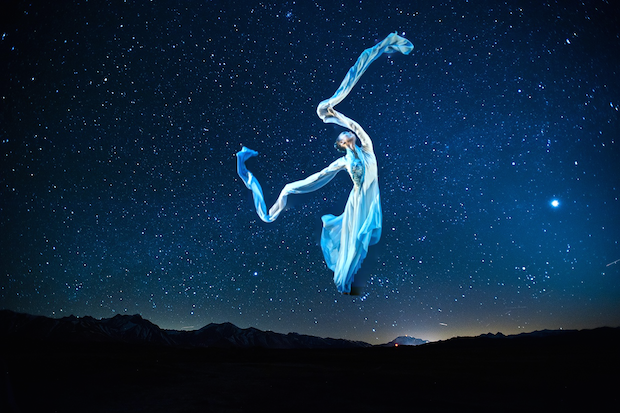
After Blending
Compare Poisson blending and Laplacian stack blending
The following is a comparison of Poisson blending and laplacian stack blending. By comparing the Poisson blending and laplacian stack blending in this case. We can see that Poisson blending a clearer edges while laplacian stack blends edges more softly. Poisson blending helps to cleanup the original background color from source image completely but is this case makes the edge too sharp. However, laplacian stack blending provides a more smooth transition for edges and thus works better in this image specifically.

Before Blending
After Poisson blending
After Laplacian Stack Blending
Reference
HTML/CSS for this page was taken from
https://v4-alpha.getbootstrap.com/components/card/