Original Image
Sharpened Image (alpha = 0.75)
The unsharp masking technique involves subtracting a gaussian filtered version of the original image from the original image leaving only high frequency details and adding this result multiplied by an alpha coefficient back to the original image. This places more emphasis on high frequency details in the image making it appear sharper.
The equation: sharpened image = original image + alpha * (original image - gaussian filtered image)
|
Original Image |
Sharpened Image (alpha = 0.75) |
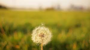
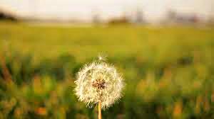
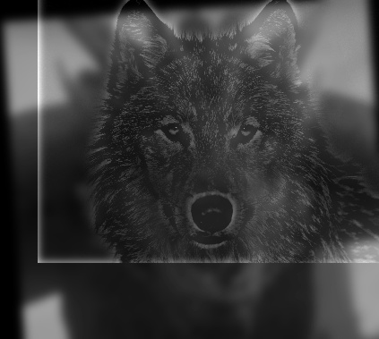
We can create hybrid images by taking the high frequencies of one image and combining them with the low frequencies of another image. The resulting hybrid image will appear as the high frequency image up close and the low frequency image from far away. We low-pass filter one image by gaussian filtering it. We then high-pass filter another image by taking that image and subtracting a guassian filtered version of that image from it. Then, we average the results that are returned from the high-pass and low-pass filters for the two images to get a hybrid. The sigma value of the gaussian filter determines the threshold of frequencies that pass through the high and low pass filters. In addition to showing a few hybrid examples, we also show the log magnitude of the Fourier transform of the two input images, the filtered images, and the hybrid image for the first example.
For all of the examples, I used a sigma of 5 for both the low-pass and high-pass filters.
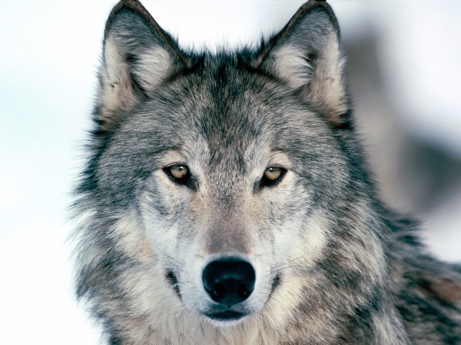
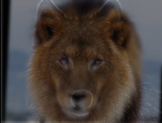
Wolf |
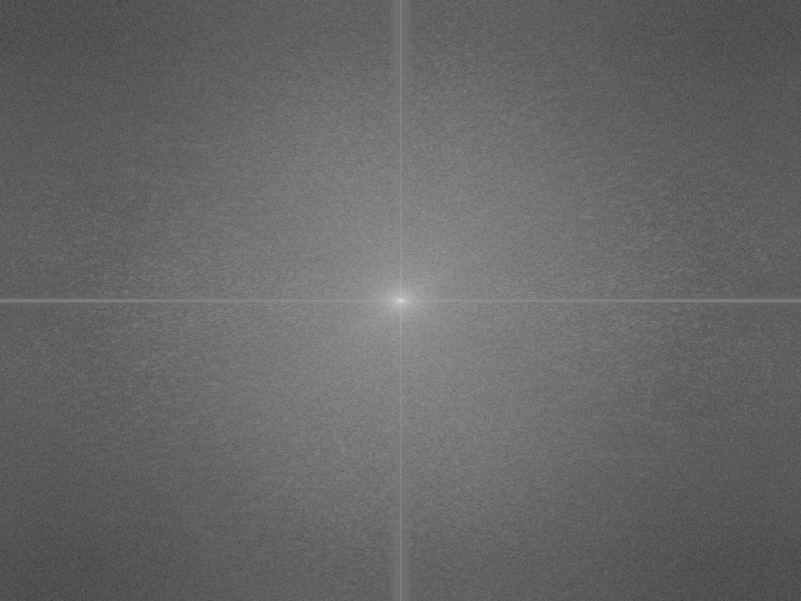
2D Fourier Transform of Wolf |
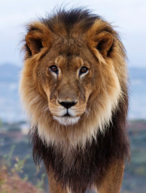
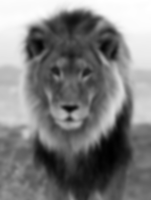
Lion |
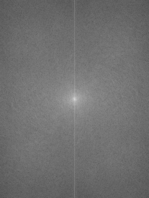
2D Fourier Transform of Lion |
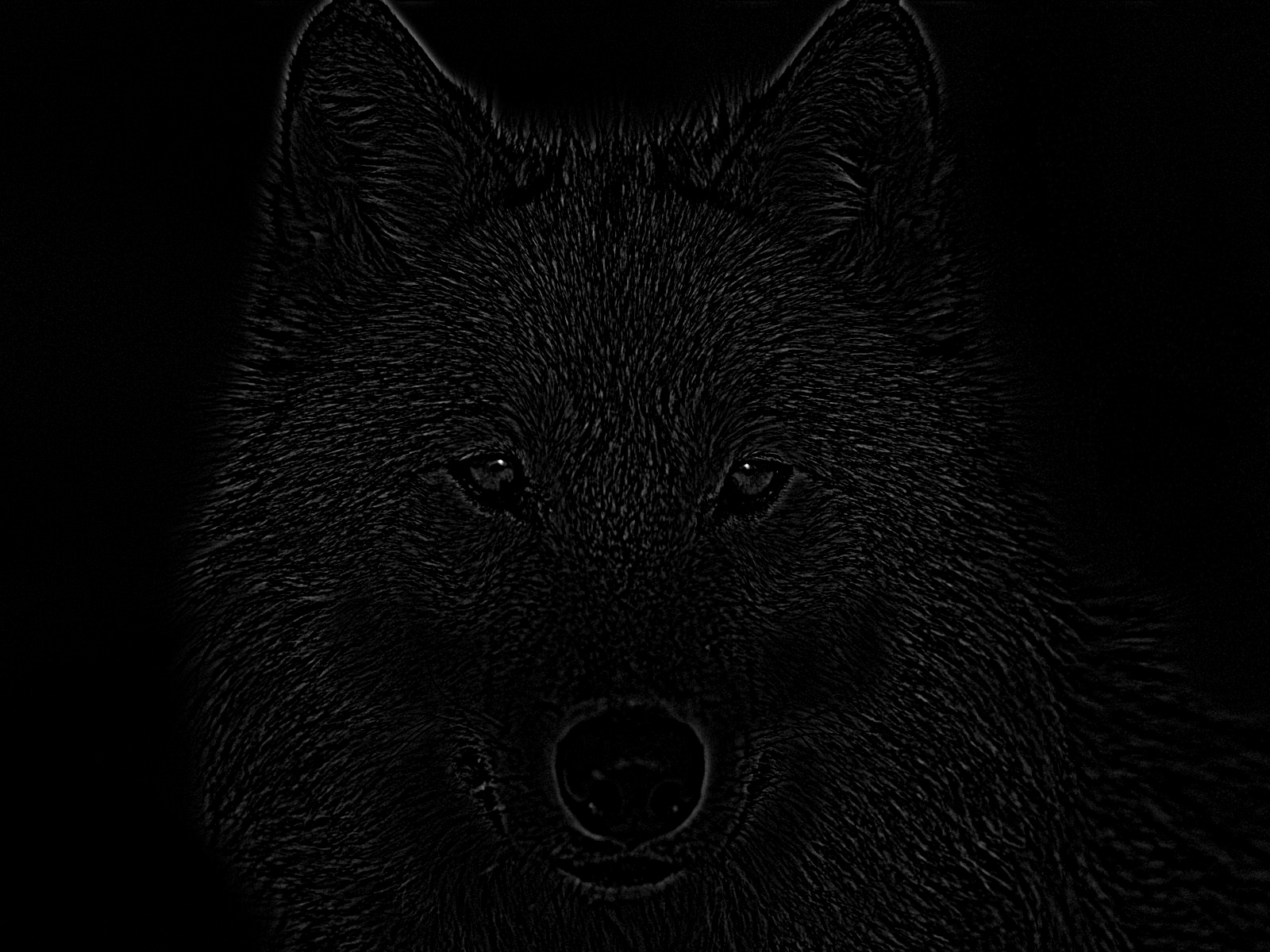
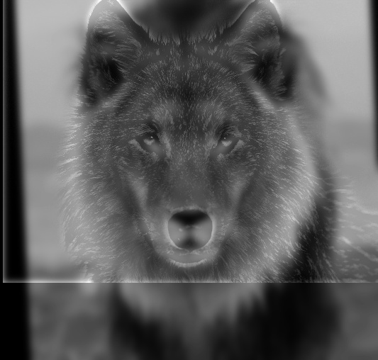
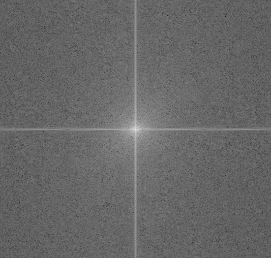
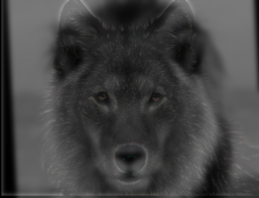
High-Pass Filtered Wolf |
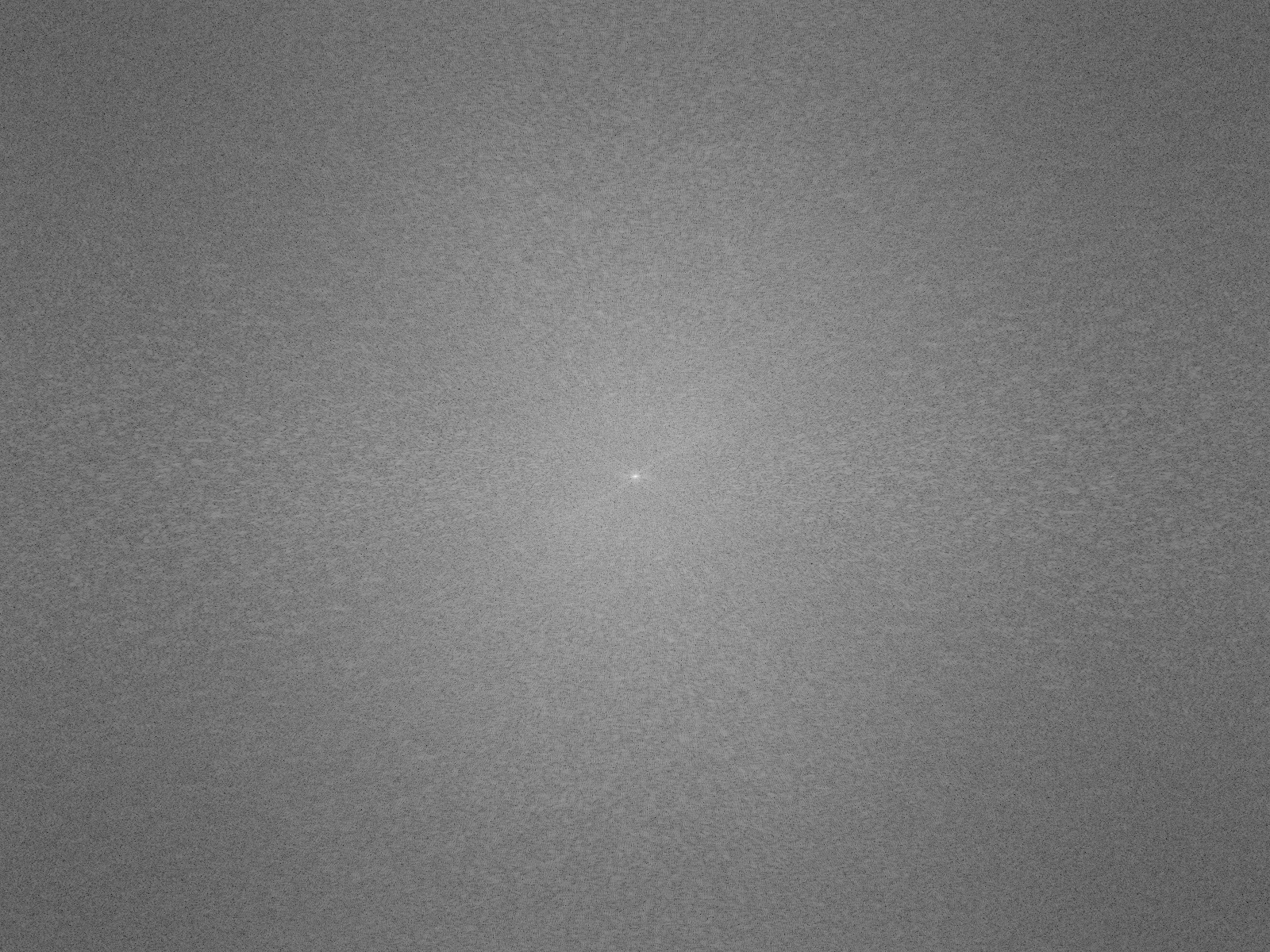
2D Fourier Transform of Filtered Wolf |
Low-Pass Filtered Lion |
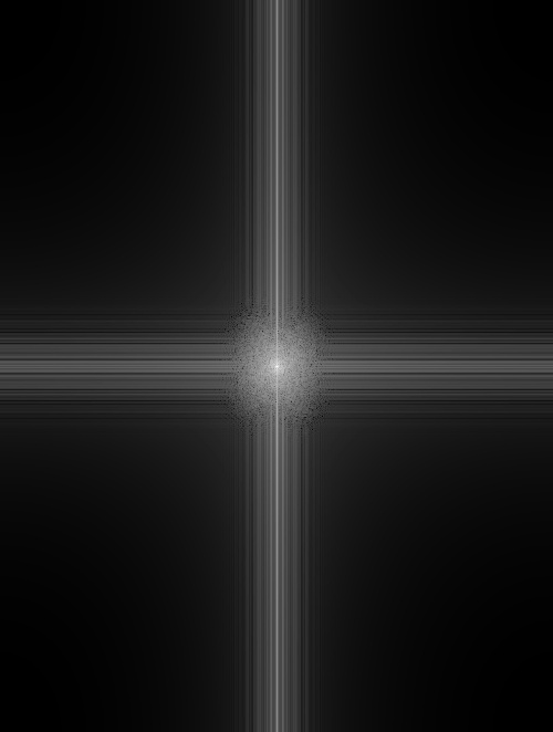
2D Fourier Transform of Filtered Lion |
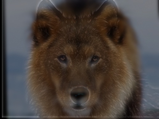
Wolf/Lion Hybrid |
2D Fourier Transform of Wolf/Lion Hybrid |
The example below is a failure, probably because the witch and forest pictures don't have similar features. This prevents us from properly aligning the images.
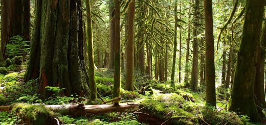
Forest |
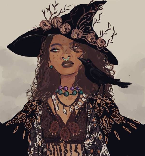
Witch |
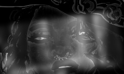
Witch/Forest Hybrid |
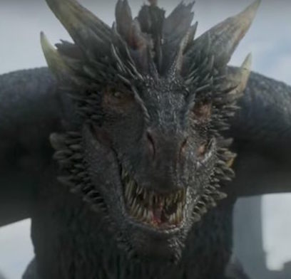
Dragon |
Wolf |
Wolf/Dragon Hybrid |
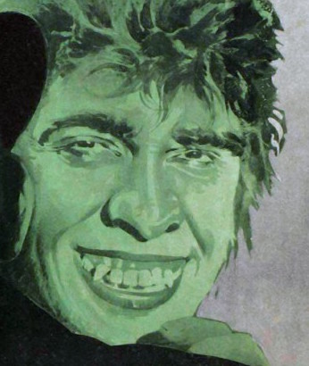
Hyde |
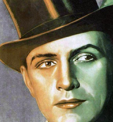
Jekyll |
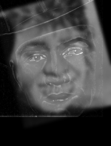
Jekyll/Hyde Hybrid |
I experimented with adding color to the high-frequency picture, the low-frequency picture, and both. Adding color to the low-frequency picture had a much stronger impact on the hybrid's coloring than adding to the high-frequency picture. Adding color to both pictures produces a similar result to just adding color to the low-frequency picture.
Color added to Low-Frequency Pic |
Color added to High-Frequency Pic |
Color added to Both Pics |
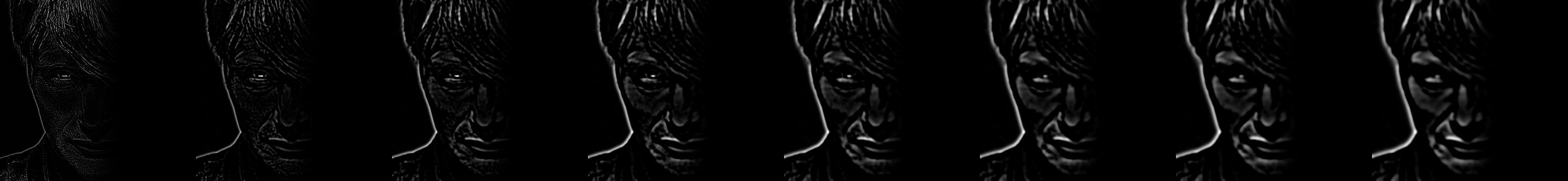
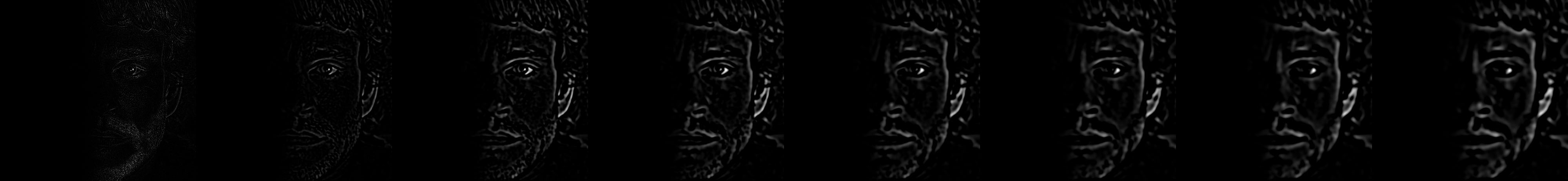
To create a gaussian stack, we gaussian filter the given image with a sigma of 2 for each level. We create a laplacian stack by taking the difference between levels of the gaussian stack. Below, is the gaussian and laplacian stack for the wolf/lion hybrid image.
|
Wolf/Lion Hybrid |
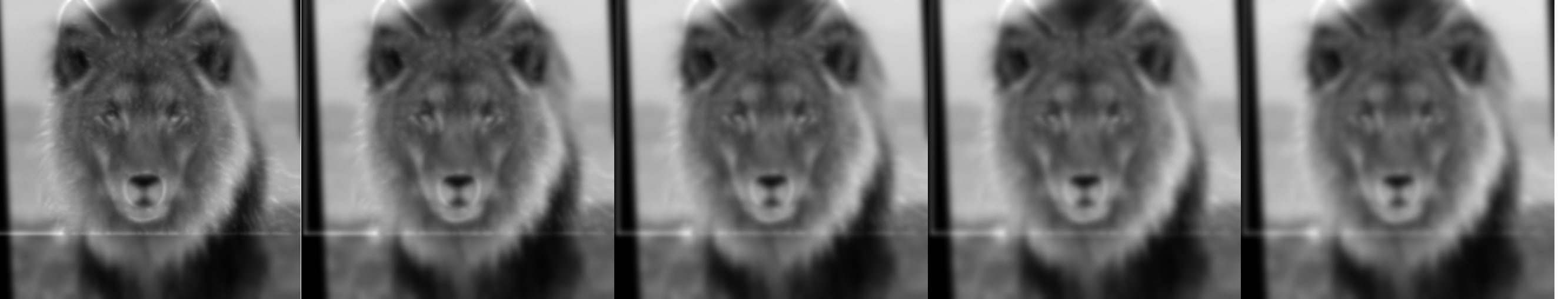
Gaussian Stack for Wolf/Lion Hybrid |
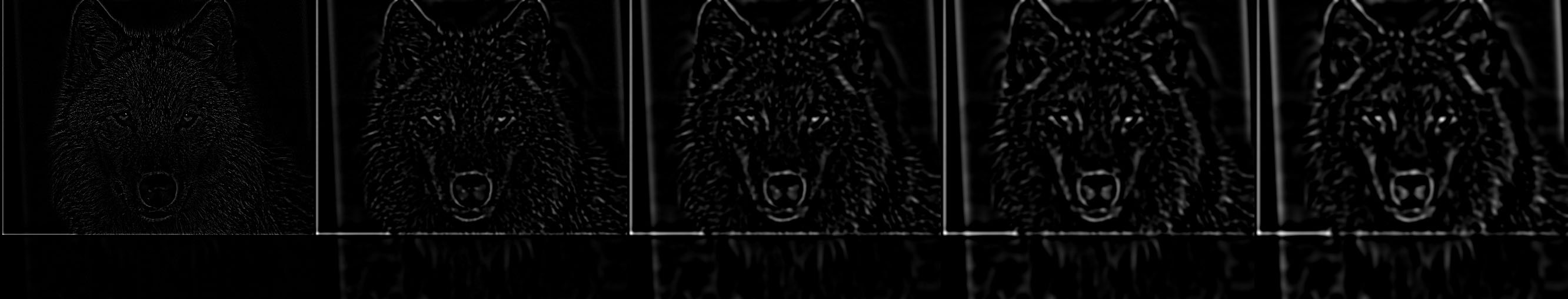
Laplacian Stack for Wolf/Lion Hybrid |
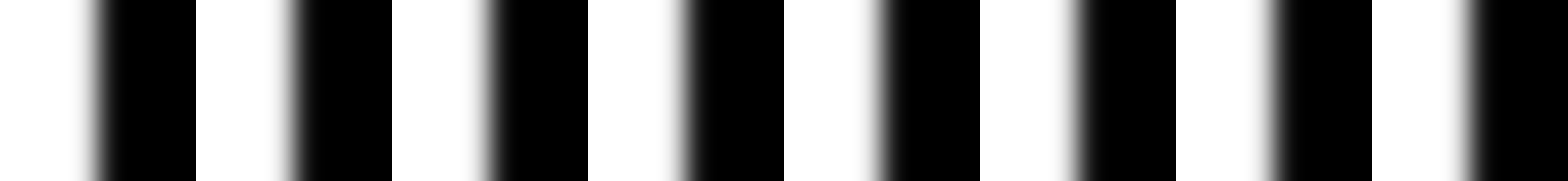
For multiresolution blending, we created laplacian and gaussian stacks for two images and a gaussian stack for a mask. For every level of the laplacian stack for both images, we multiplied the corresponding level of the gaussian mask stack with one image and 1 minus the gaussian mask stack level with the other image. We added all of these results together for all the levels along with the image on the last level of the gaussian stack for both images multiplied by the last level of the gaussian stack for the mask and 1 minus the last level of the gaussian stack for the mask. To get a more gradual seam, I initially gaussian filtered every mask I used with a sigma of 30 before creating a gaussian stack.
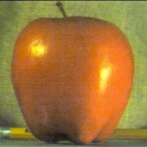
Apple |
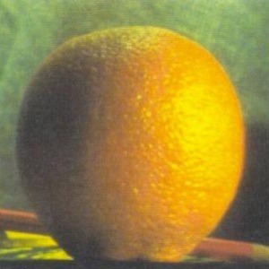
Orange |

Mask |
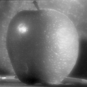
Oraple |
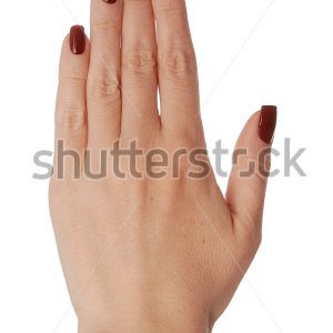
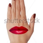
Hand |
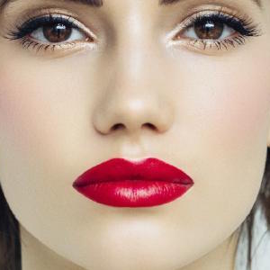
Lips |
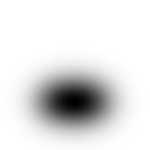
Irregular Mask |
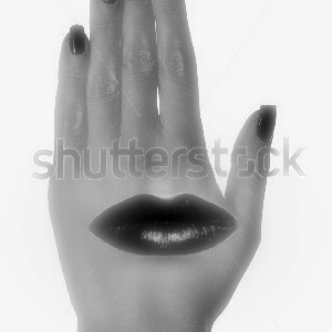
Lip/Hand Blend |
For this blend, I also show the laplacian stacks for the two masked images seperately and the blended result. The blend could have been better if the facial features of the two faces were more level with each other.
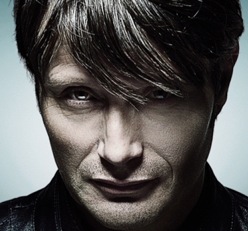
Hannibal |
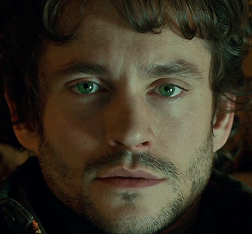
Will |

Mask |
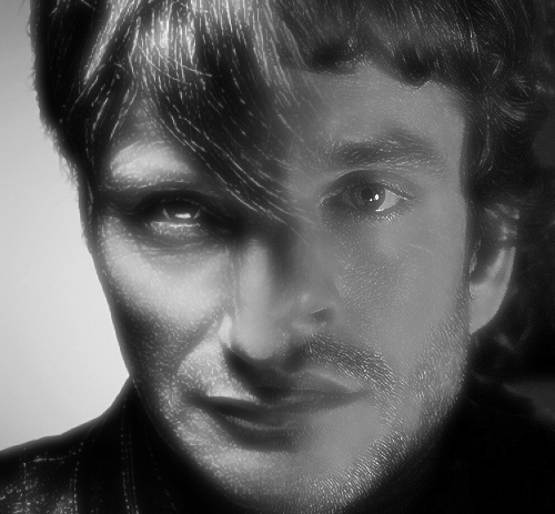
Hannibal/Will Blend |
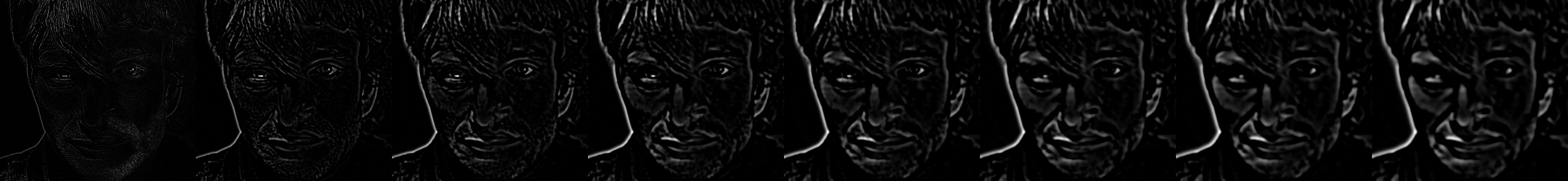
Combined Image Laplacian Stack |
Masked Hannibal Image Laplacian Stack |
Masked Will Image Laplacian Stack |
Mask Gaussian Stack |
Here is an example of a colored blend image. Below we use color on the hand/lips blend.
|
Hand |
Lips |
Irregular Mask |
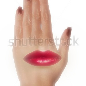
Lip/Hand Blend |
In this section of the project, we attempt to implement poisson blending in order to seamlessly blend a source image into a target image. Simply copy and pasting creates visual seams, so we attempt to preserve the gradients of the source image without changing the value of the background pixels in the target image. Preserving the gradients preserves the structure of the source image which is more important than matching the exact pixel intensities. Attempting to preserve the gradients of the source image while preserving the background pixel intensities of the target image can be written as a least squares problem Ax=b. We create 3 b vectors for each color channel. Each column of A represents a pixel in the final image and we set up an equation for each pixel as well so each row in A also represents a pixel. For any pixels outside a source region/mask, we set the corresponding column in A to 1 and 0s everywhere else for the corresponding row and we set the corresponding row in each of the 3 b vectors to the value of the target image in each color band. For each pixel inside the source region/mask, we set the corresponding column of the corresponding row in A to 4 and set -1 for each of the pixel's four neighbors (up, down, left, right). For the corresponding row in the 3 b vectors we set it equal to 4*(intensity of current pixel in source image) minus all the intesities of the four neighboring pixels in the source image for each color channel. Solving this Ax=b equation gives us a new image that looks well blended. The minimization function that we used to make the Ax=b equation for poisson blending is available on the course website.
Before doing poisson blending, we start with the simple problem of reproducing an image by matching its gradients and the matching the value of one corner pixel. Below are the original and reproduced images.

Original Image |
Reproduced Image |
Using the methodology provided in the overall project description, we were able to implement poisson blending, and a few examples are shown below. I solved an Ax=b equation where every pixel outside the masking region has a row where that pixel's position is set to 1 and the corresponding row in b is set to the intensity of the target image while each pixel inside the masking region is compared to its four neighbors and the differences between the pixel and its neighbors is equal to the differences between the pixel and neighbors in the corresponding source image, so the gradients are preserved.
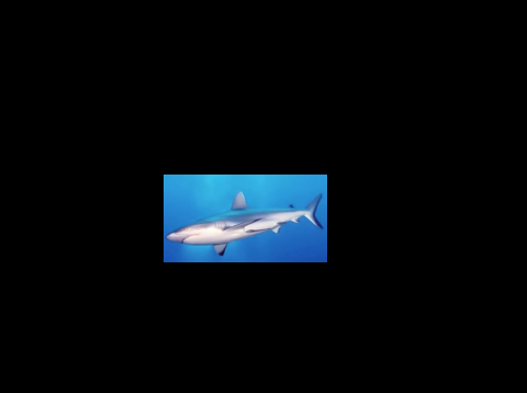
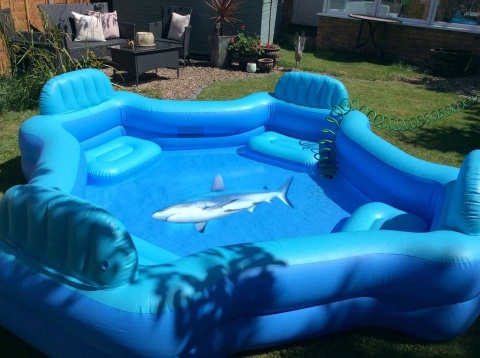
Source Image |
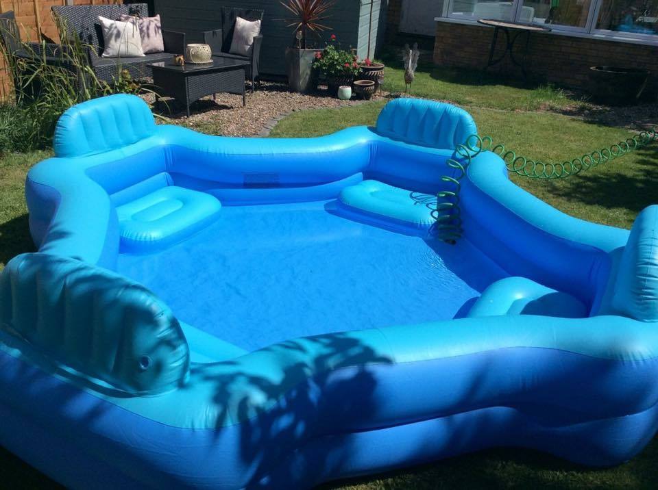
Target Image |
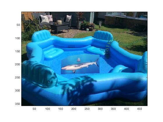
Source Copied Into Target |
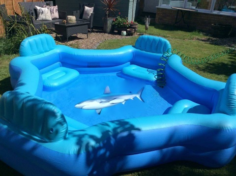
Shark/Pool Blended Result |
As described in the project description, we attempted to match the gradients of the source image while preserving the pixel intensities of the target image for the background. Since the background of the shark image and the pool have similar coloring, the poisson blending works very well for this example.
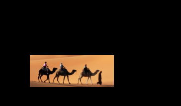
Source Image |
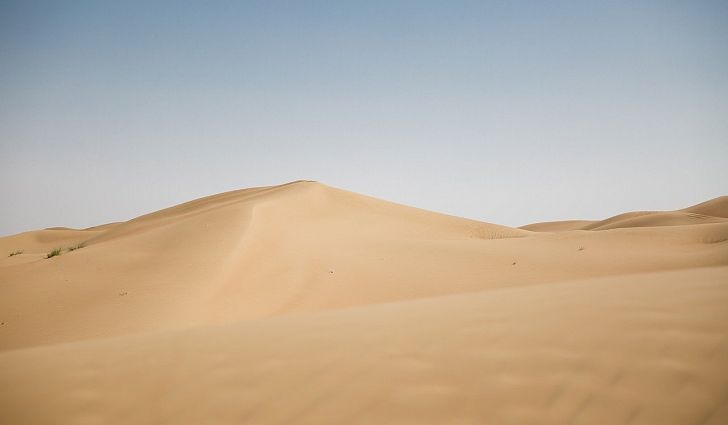
Target Image |
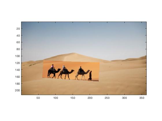
Source Copied Into Target |
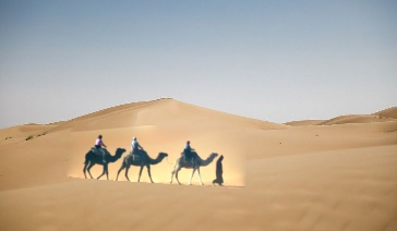
Camel/Desert Blended Result |
This example also blends successfully, but could have been better if the background of the source image was more similar to the corresponding region in the target image.
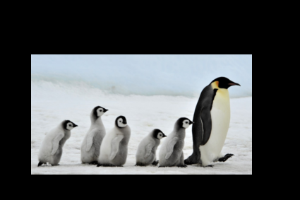
Source Image |
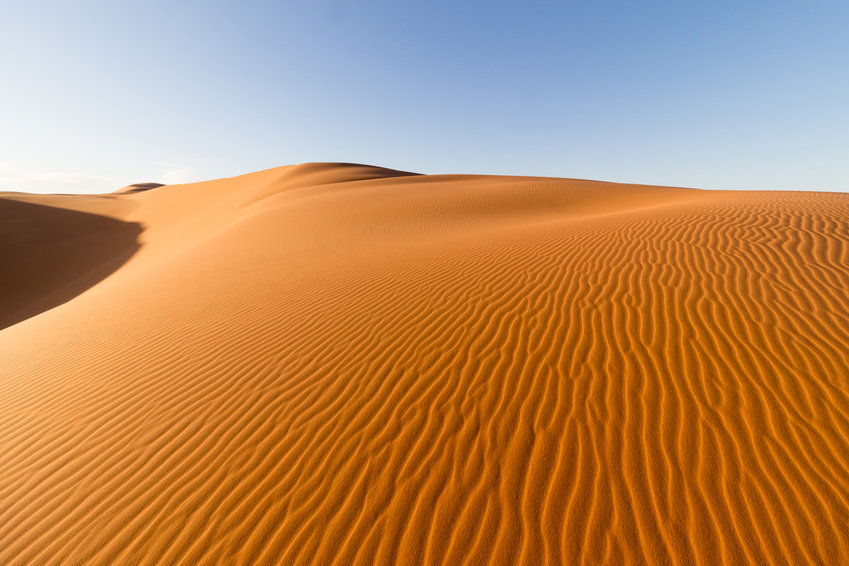
Target Image |
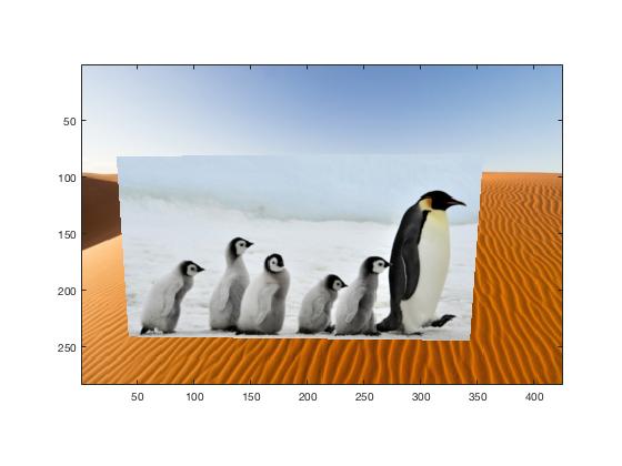
Source Copied Into Target |
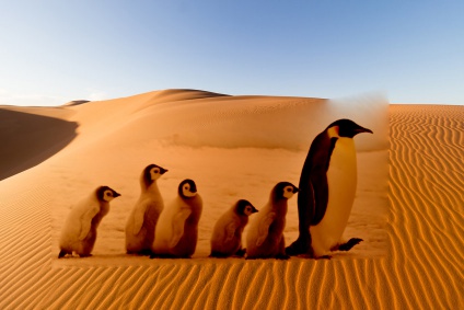
Penguin/Desert Blended Result |
This example is a failure because the pixel values of the source image are so different from that of the target image. Thus, in the attempt to maintain source gradients as well as the pixel values of the target image, the penguins are turned orange like the desert. The vast difference between the source and target images also causes the seam to visible at some points.
For extra credit, I also implemented mixed gradients, which is like poisson blending, but for each gradient in the source region, we preserve the gradient that is higher between the source and target image. This does not change the A matrix but it does change the b matrix for all 3 color channels. The value of the b matrices depend on whether the absolute value of the target gradient is greater than the absolute value of the source gradient. An example of mixed blending is shown below.
|
Source Image |
Target Image |
Source Copied Into Target |
Shark/Pool Mixed Blended Result |
For the hands and lips images that we used for multiresolution blending, we also attempted to blend these two images using poisson blending and mixed blending. Overall, the poisson blending and mixed blending techniques worked better than the multiresolution blending probably because the background of the lips image, which has a skin color, was similar to the color in the hand image, which was also skin colored. Thus, preserving gradients of the source image/target image preserved the structure and color of the original source image. I believe that multiresolution blending would work better in cases where the backgrounds of the source and target are very different and the mask is less irregular.
|
Hand |
Lips |
Lip/Hand Multiresolution Blend |

Lip/Hand Poisson Blend |
Lip/Hand Mixed Blend |