Project 3: Fun with Frequencies and Gradients
cs194-26-aeoGenevieve Tran
Part 1.1: Warm-Up
The image sharpening technique is accomplished by using a gaussian filter to create a blurred version of the original image. We then create a high-pass version of the image by taking the difference between the original image and the blurred image. Once we extract the high-passed filtered image, we can add it back to the original image with an appropriate weight (alpha) to get a sharpened version.

Original image

Alpha = 1
Alpha = 5
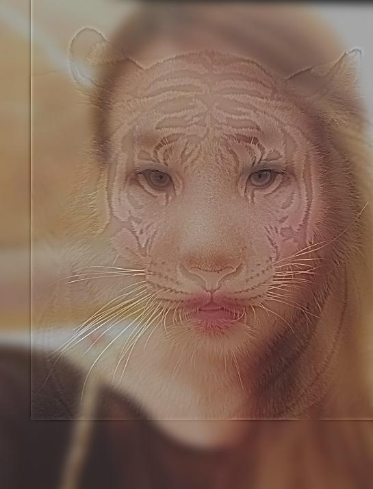
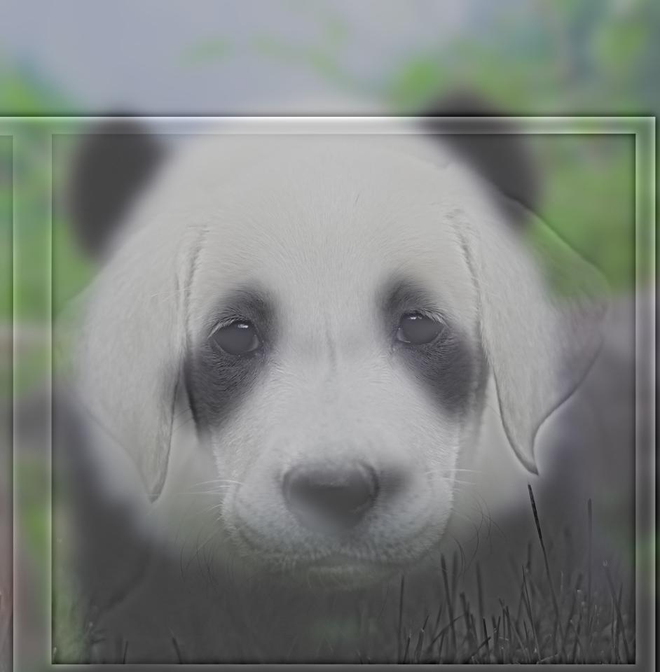
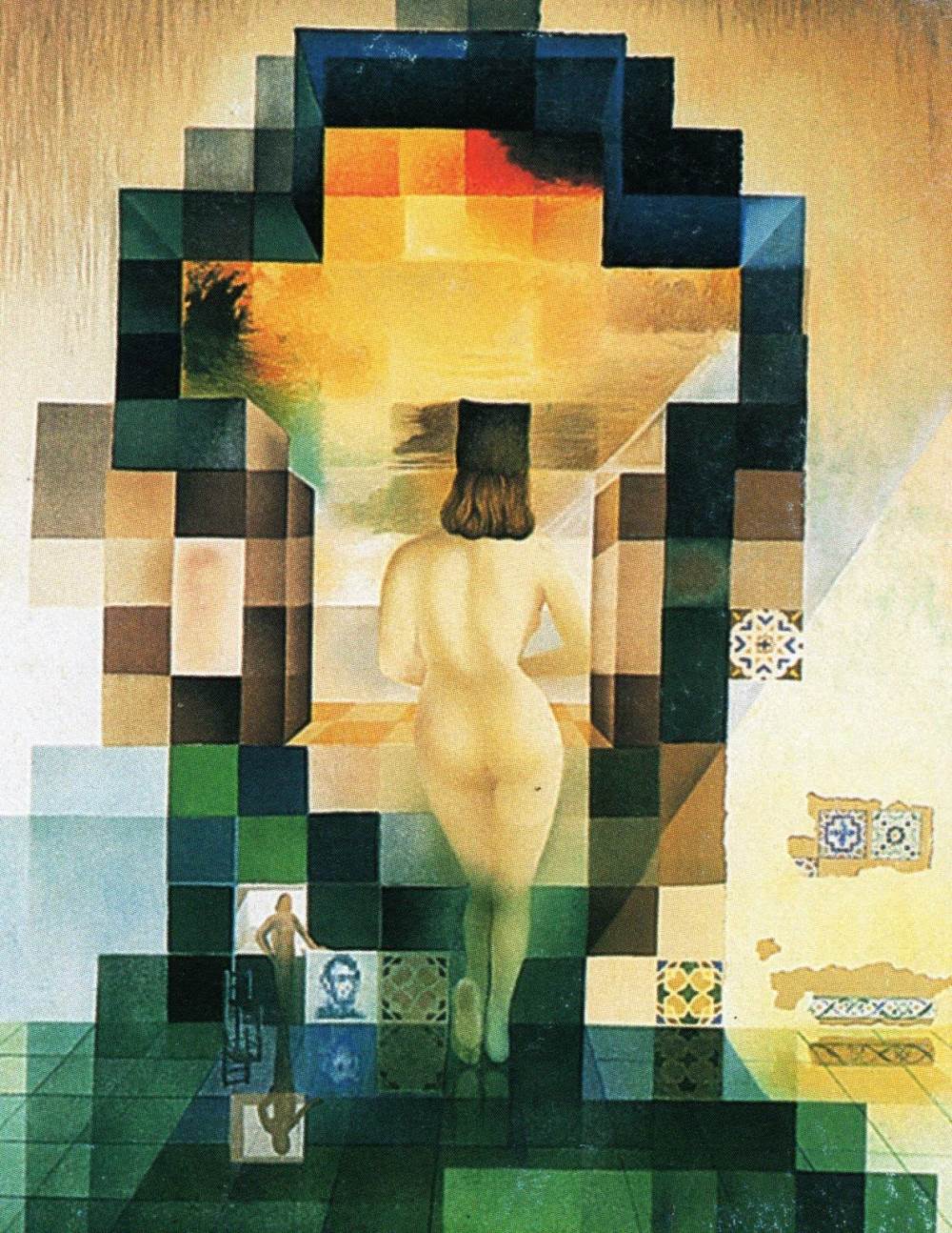
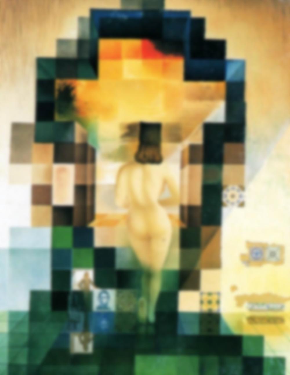
Part 1.2: Hybrid Images
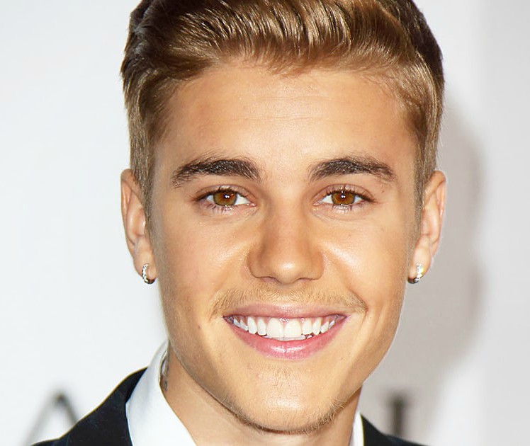
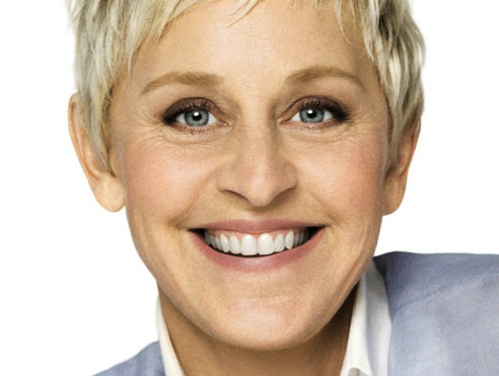
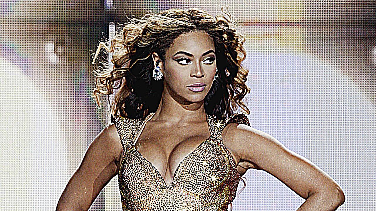
Published at SIGGRAPH 2006, Hybrid Images (Oliva, Torralba, and Schyns) documents an approach to creating static images that change in appearance based on the distance of the viewer from the image. In this assignment I created such hybrid images by blending the high-frequency portion of one image with the low-frequency portion of another.
The main parameter to tune was the cutoff frequency  . I measure frequency in cycles/image. In order to extract the low frequencies in one image, I convolve the input image with a Gaussian function,
which acts as a low-pass filter. Likewise, I extract the high frequencies from another image using a Laplace filter, which I obtained by taking the difference of the input image and the input convolved with a Gaussian.
I chose a filter sigma as follows:
. I measure frequency in cycles/image. In order to extract the low frequencies in one image, I convolve the input image with a Gaussian function,
which acts as a low-pass filter. Likewise, I extract the high frequencies from another image using a Laplace filter, which I obtained by taking the difference of the input image and the input convolved with a Gaussian.
I chose a filter sigma as follows:
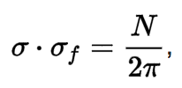
Where N is the number of pixels along the width axis of the image. This formula is taken from the Wikipedia article on the Gaussian Filter.
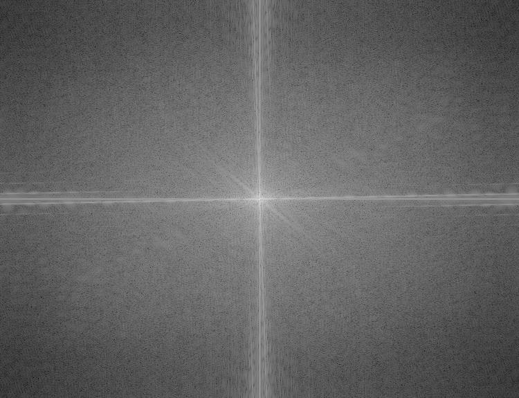
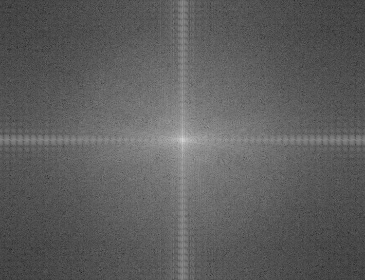
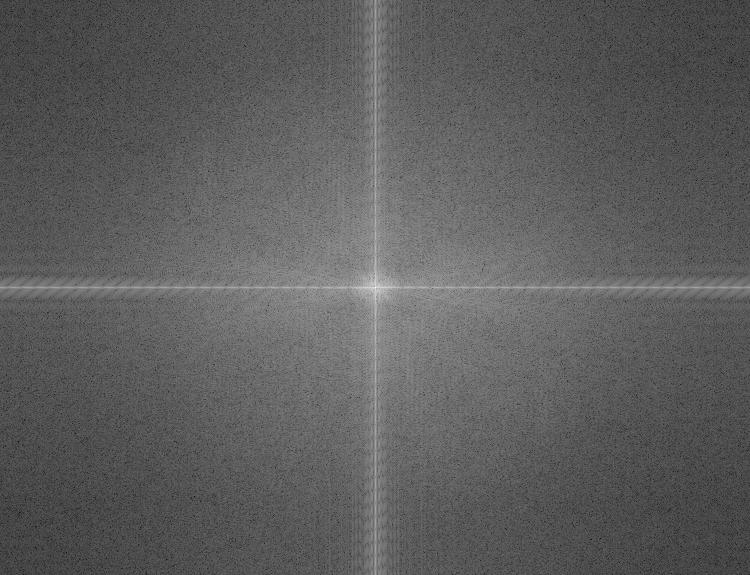
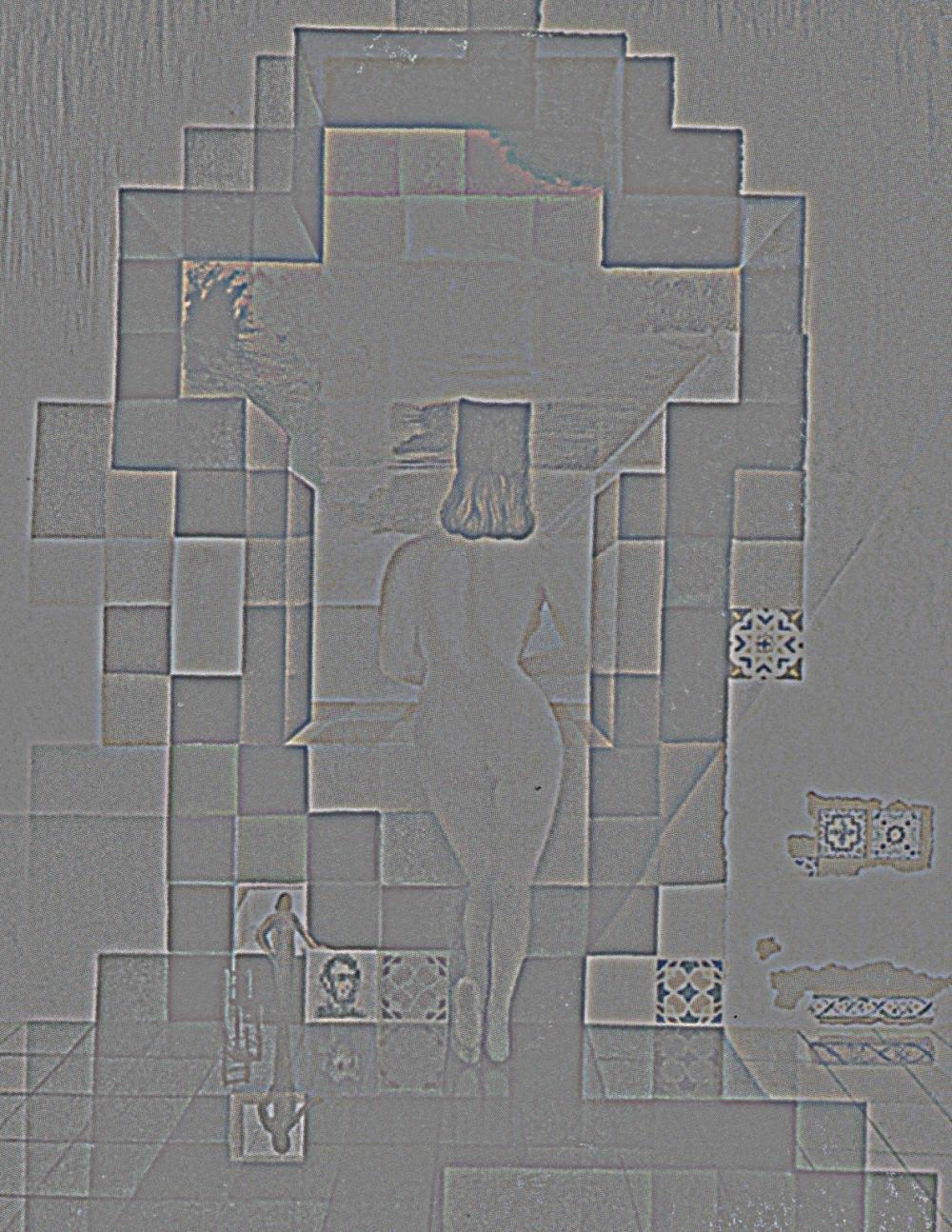
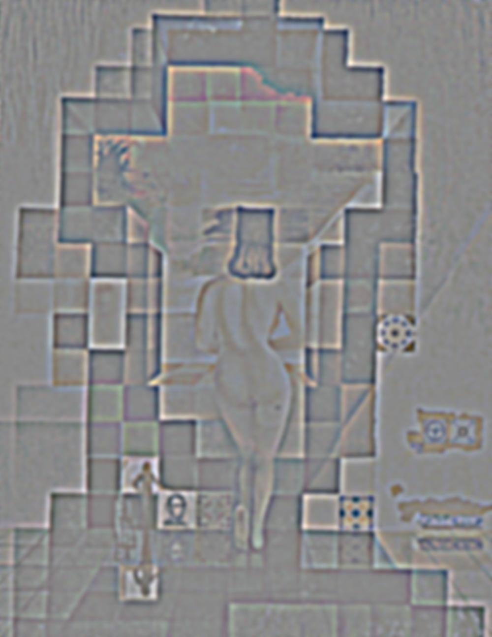
Below you find the outline of the procedure with the processed images on the left and the log magnitude of the Fourier transform on the right of the chosen hybrid. The chosen high frequency cut-off for the first image is 36 cycles/image. The chosen low frequency cut-off for the first image is 16 cycles/image.
Procedure:Align Images. This was done based on the skeleton code provided by the staff.

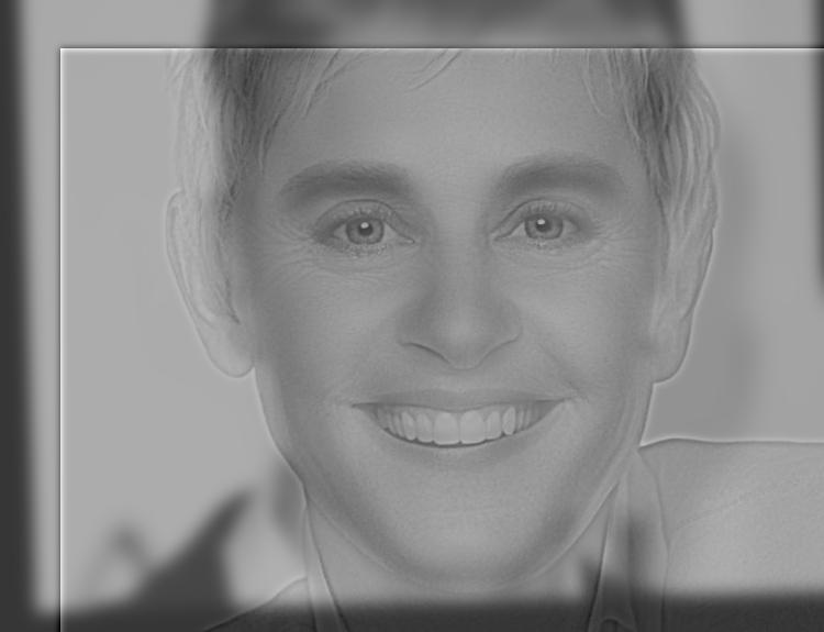
Apply a low-pass filter. Convolve the first input image with a Gaussian filter.
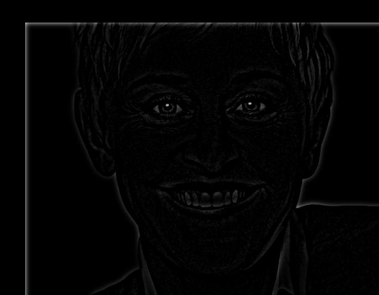
Apply a high-pass filter. Convolve the first input image with a Laplacian filter.
Add the two previous results with weights of 0.5 each.
More Results
Robin and Dominic Joseph. Not related. Low frequency cutoff = 16, high frequency cutoff=48

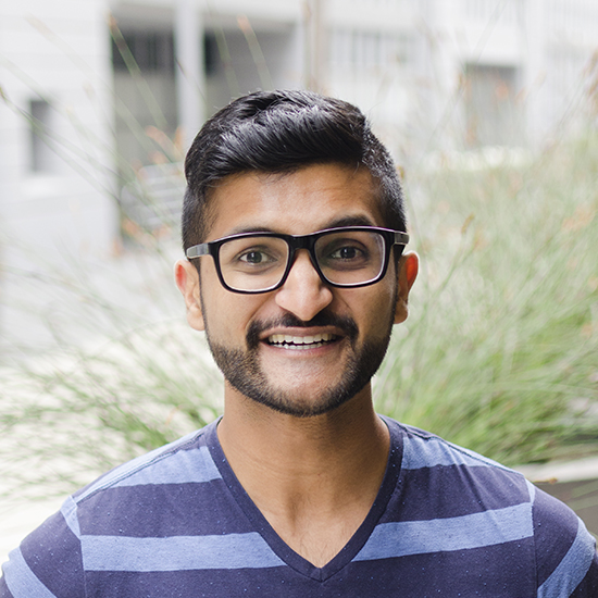
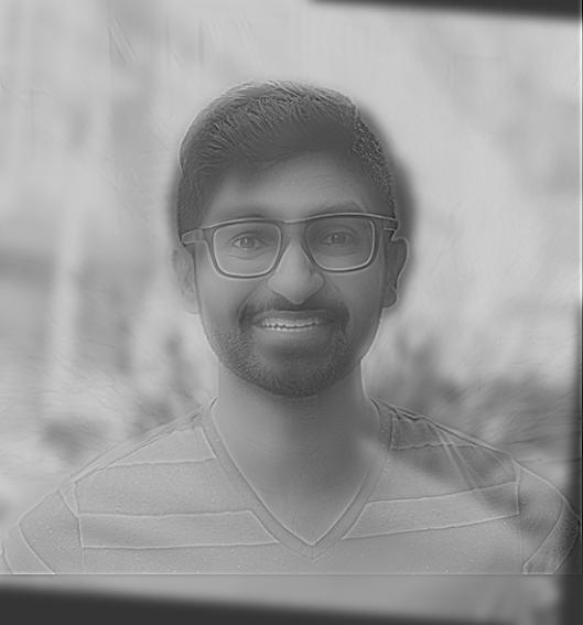
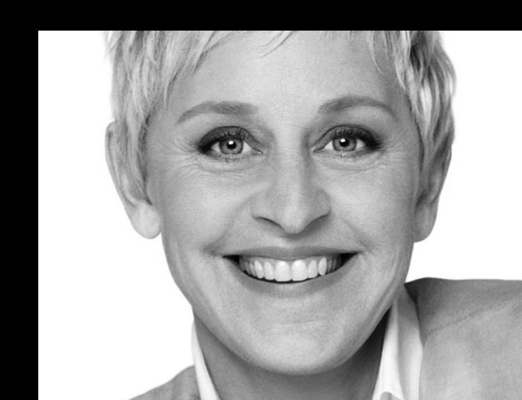
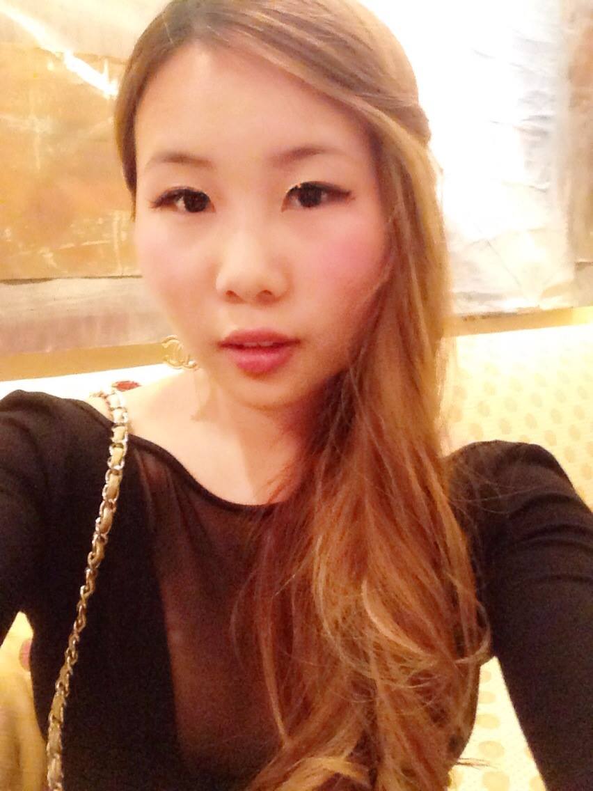
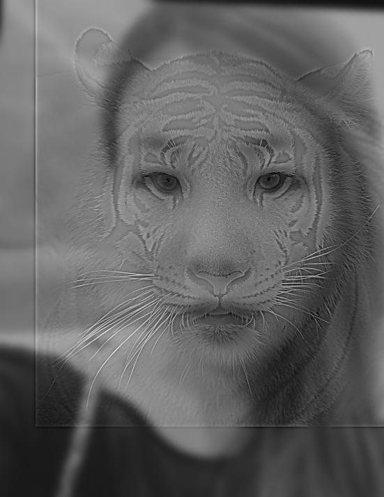
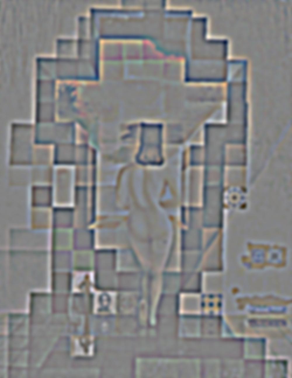
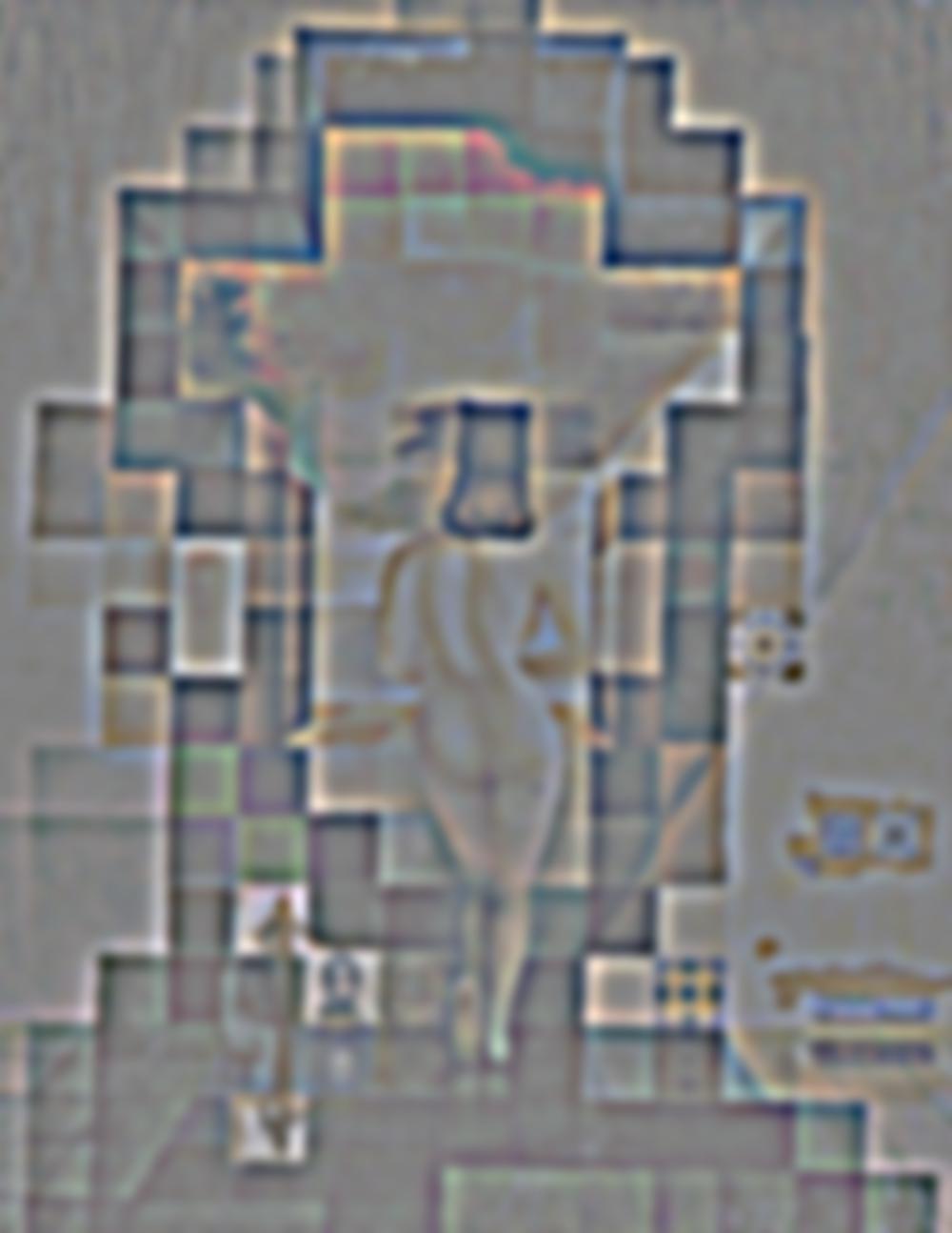
My best friend and her spirit animal. Low frequency cutoff = 16, high frequency cutoff=36
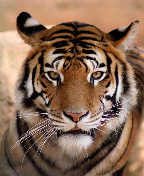
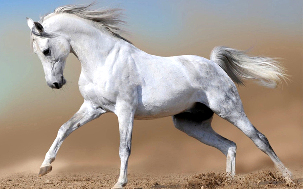
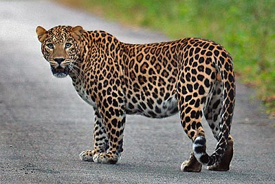
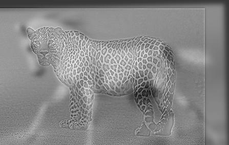
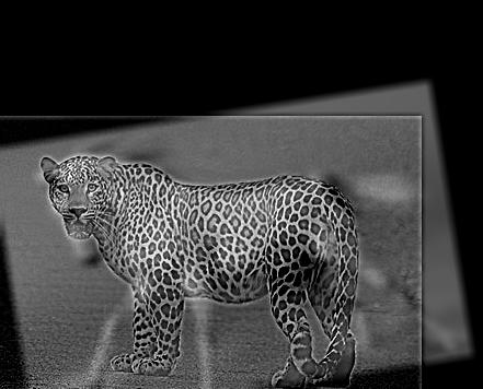
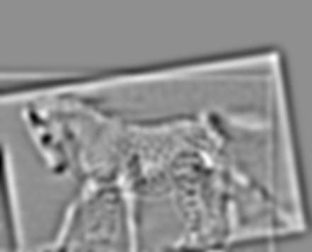
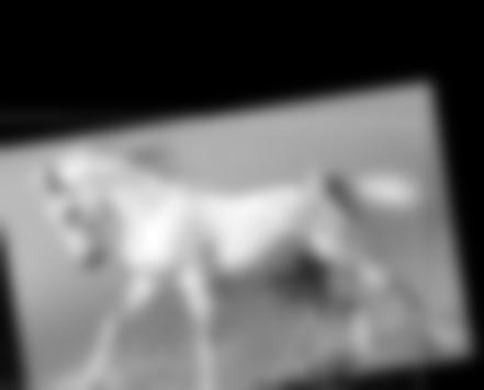
White horse and leopard. Low frequency cutoff = 16, high frequency cutoff=36
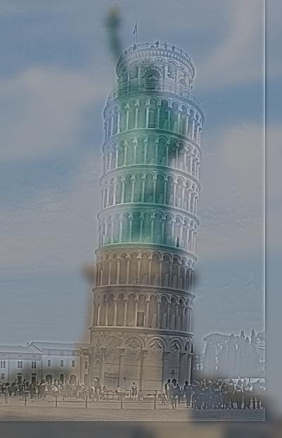
Color Enhancement
To color the image I chose to run a low pass filter on the image with color and a high pass filter on an image in grayscale. It works better because this way more of the image has color (as opposed to doing that with a high pass filtered image) and the colors from both images do not clash with each other.
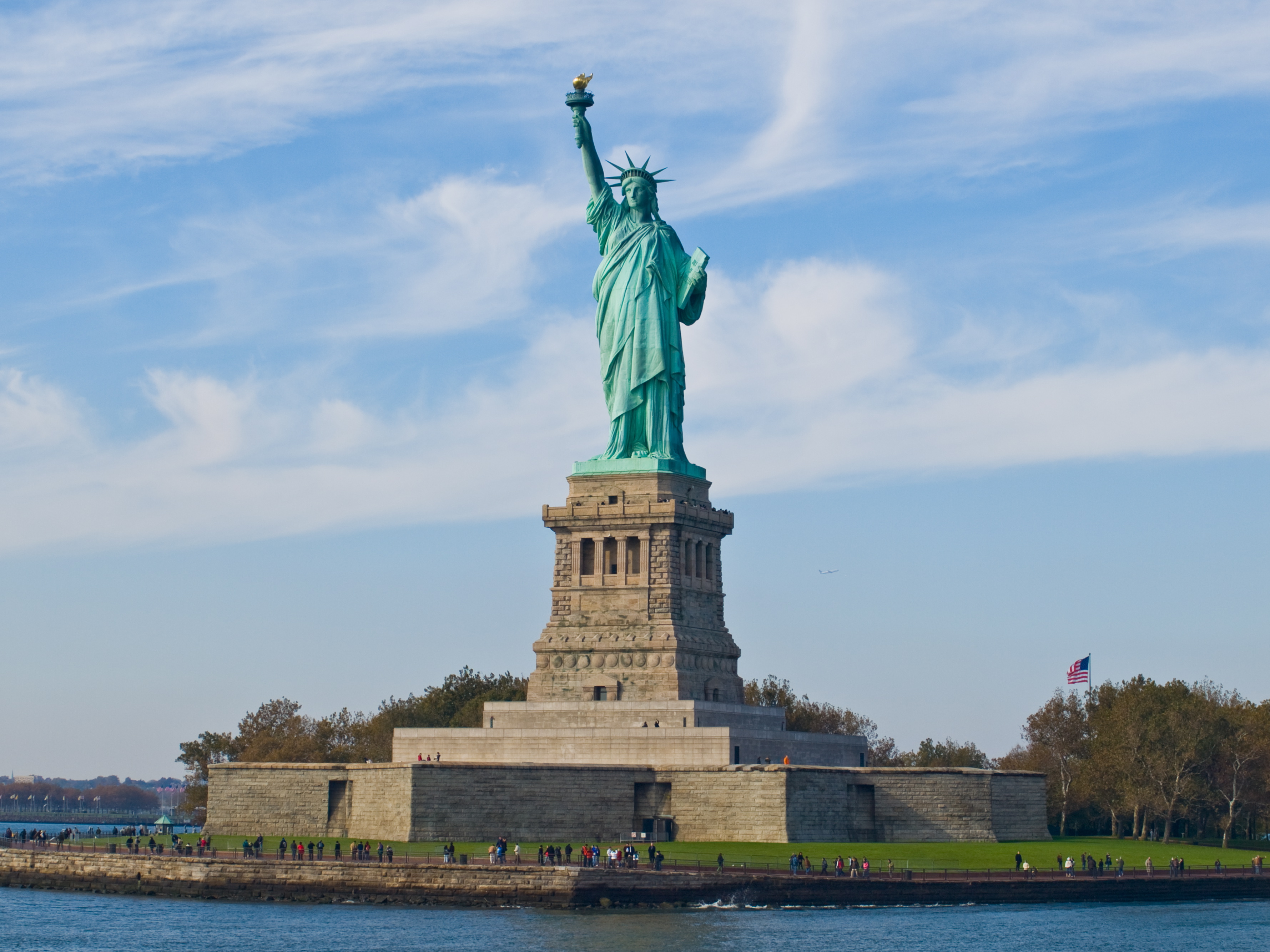
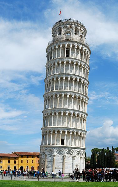
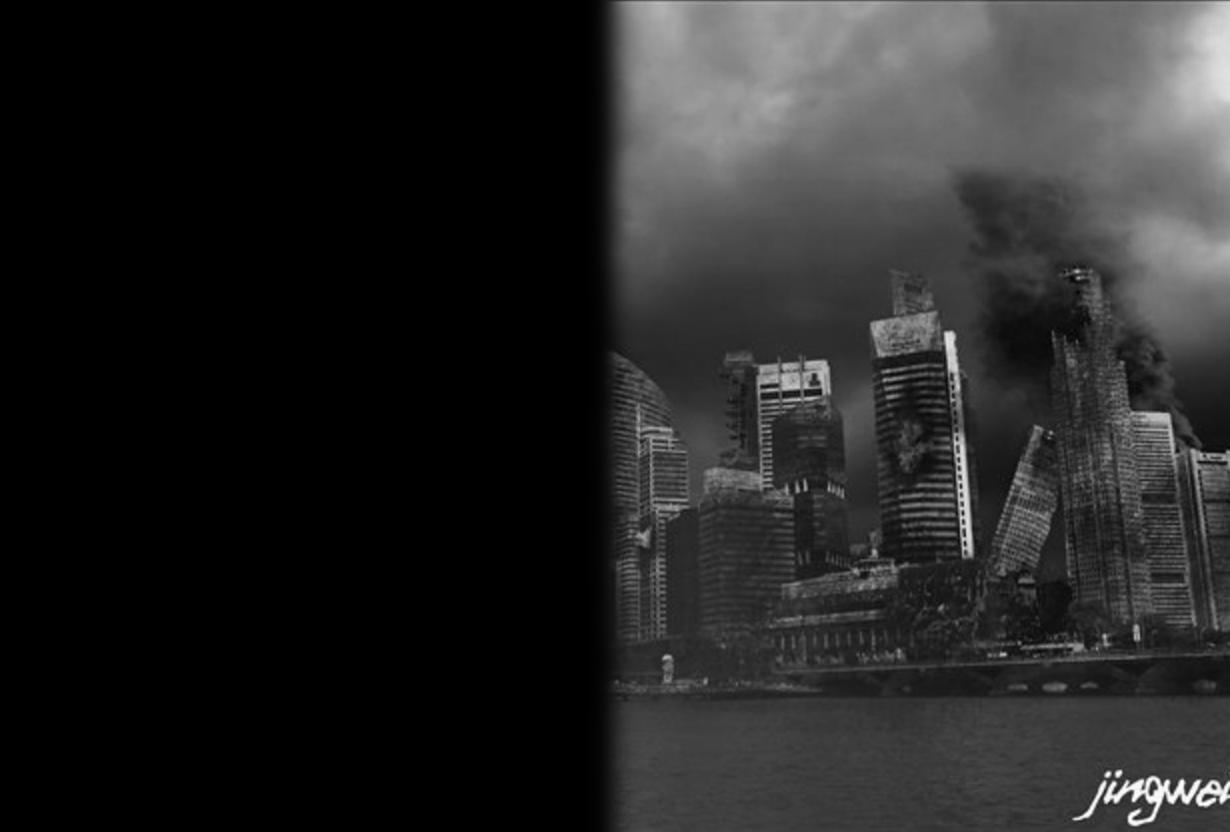
Statue of Liberty and the Leaning Tower of Pisa. Low frequency cutoff = 12, high frequency cutoff=26
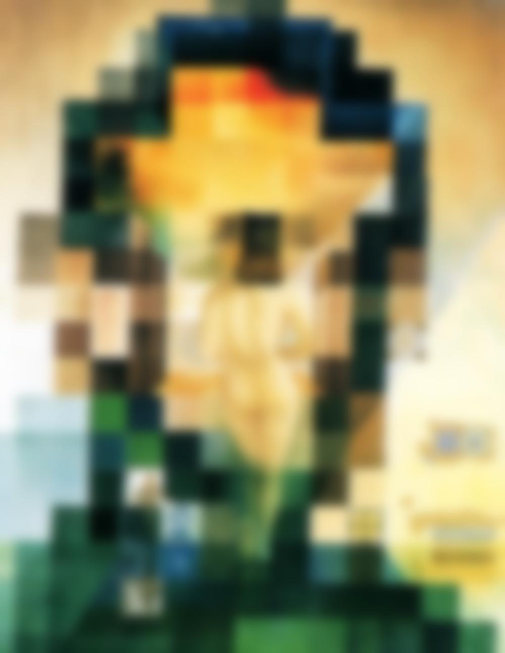
My best friend and her spirit animal. Low frequency cutoff = 12, high frequency cutoff=36
White horse and leopard. Low frequency cutoff = 12, high frequency cutoff=26
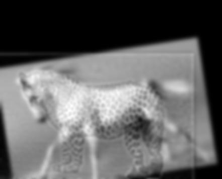
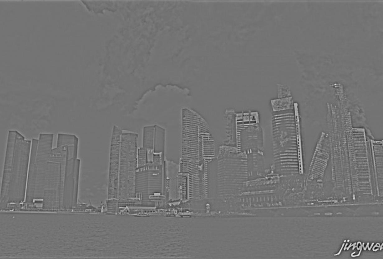
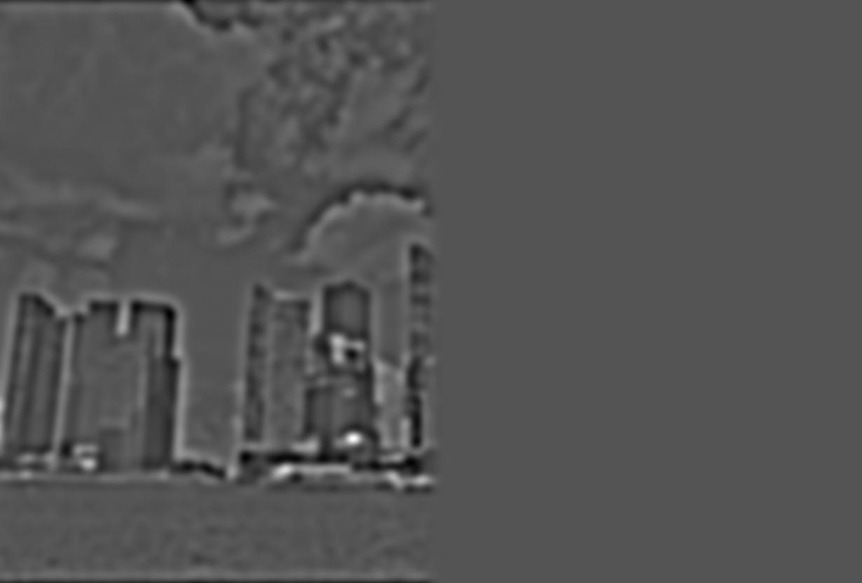
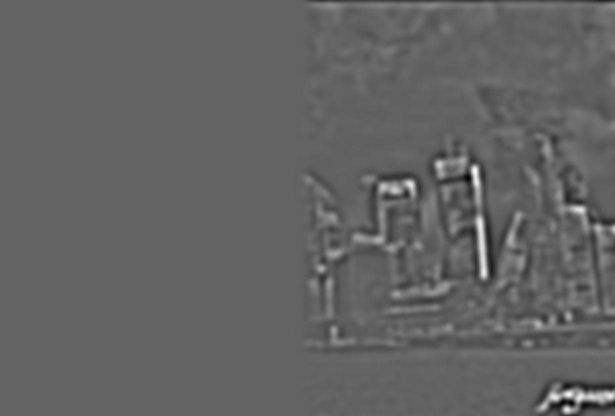
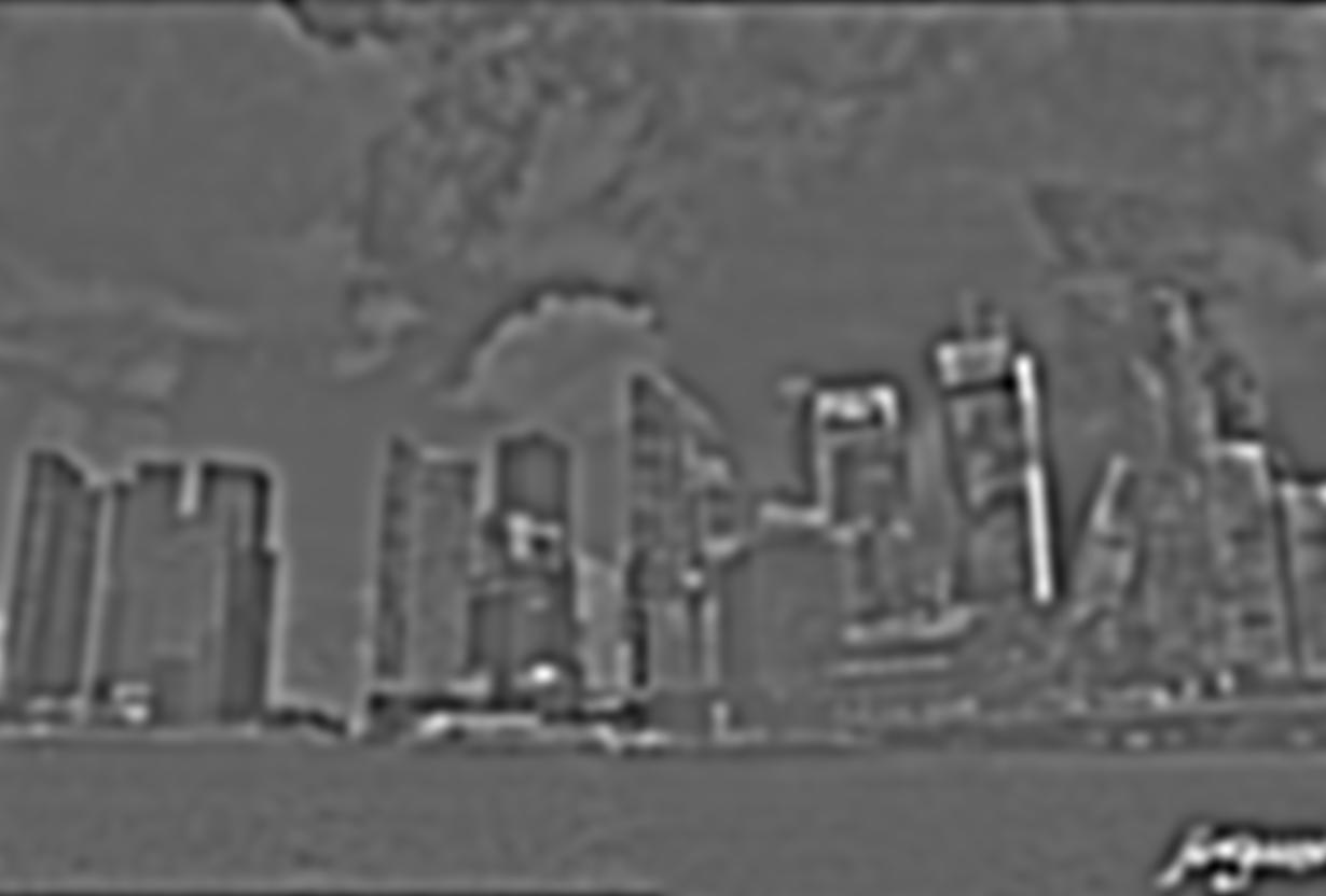
Part 1.3: Gaussian and Laplacian Stacks
Overview:In this assignment I created Gaussian and Laplacian Stacks. On the first level of the gaussian stack we have the original image convolved with a Gaussian filter of a selected sigma. The first level of the laplacian stack is just the first image of the gaussian subtracted from the original image. As we progress down the stacks we take the image from the previous level of the gaussian stack and apply a gaussian filter with the fixed sigma to it to get the next level of the gaussian stack. Similarly to get the laplacian at this level we subtract the given result from the gaussian at the previous level. The last level of the Laplacian stack is set to equal the last level of the Gaussian stack.
Original Image
Gaussian Stack (sigma = 5)


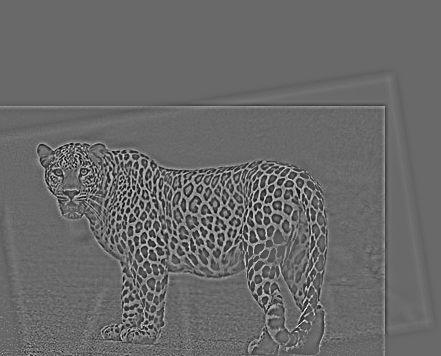
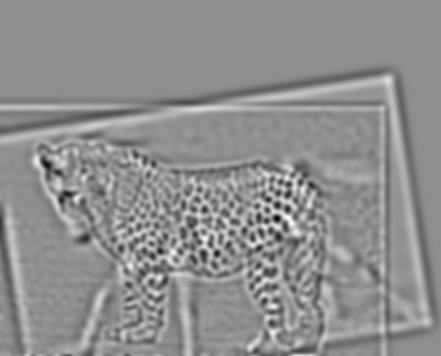
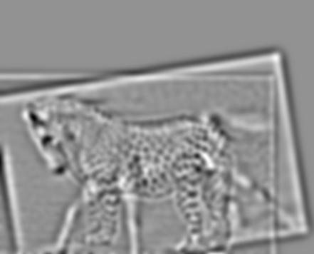
Laplacian Stack (sigma = 5)
Original Image
Gaussian Stack (sigma = 3)


Laplacian Stack (sigma = 3)
Part 1.4: Multiresolution Blending
Overview:In this portion of the homework I attempted to create smoothly blended images based on the 1983 paper by Burt and Adelson.
In order to do so, I utilized the Lalpacian stacks of the two input images. We mutliply an input
image by a mask the indicates the area of that image we want to include
in the final result by having values of 1 in that area and 0 everywhere else. By using the Laplacian,
we can blend different ranges of frequencies
of two input images. The lower we go in frequency, th blurrier the edge of the mask gets.
By creating a stack of blended laplacian-filtered images, we can create a smoother blended image.
The multi-resolution blending process uses the following equation:

Favorite Result Laplacian Analysis
High Frequency
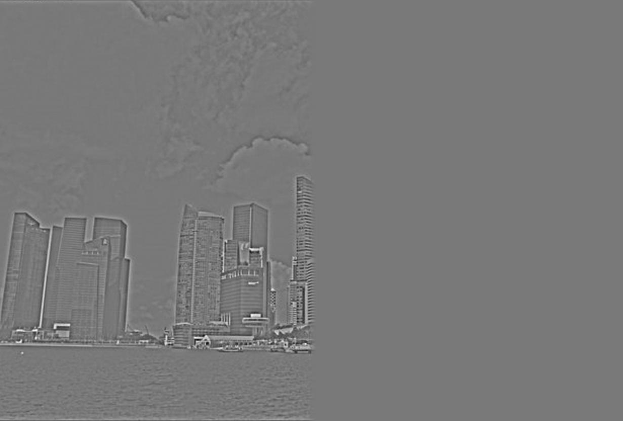
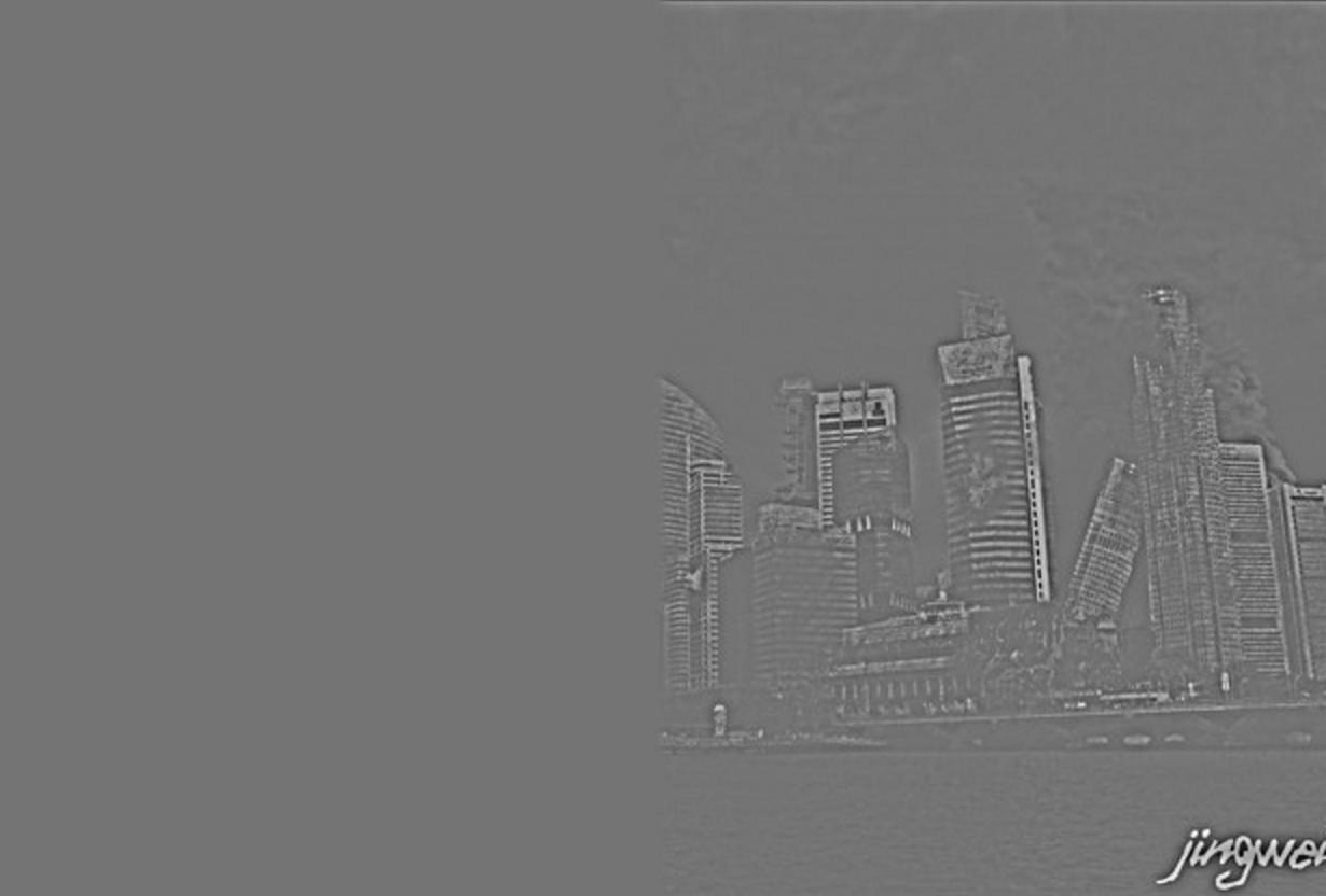
Medium Frequency
Low Frequency
Summed Images

Additional Images
|
Original Image 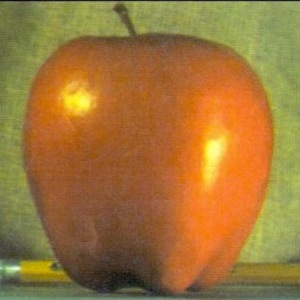
|
Original Image 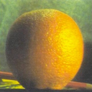
|
Mask 
|
Blended 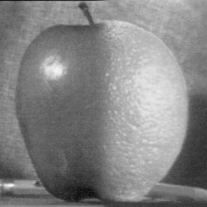
|
|
Original Image 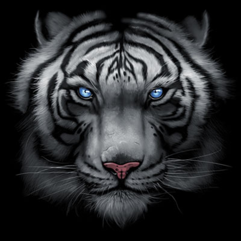
|
Original Image 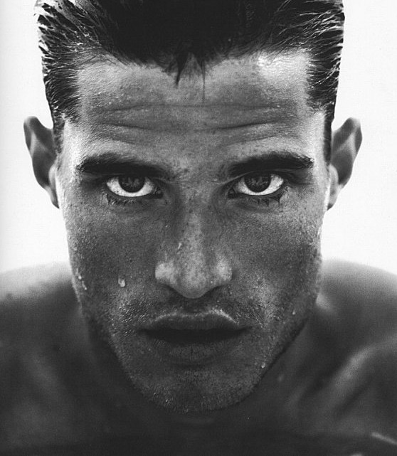
|
Mask 
|
Blended 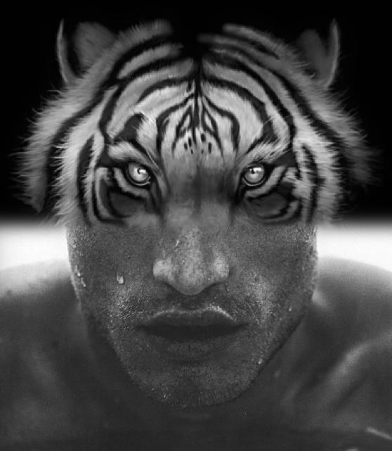
|
|
Original Image 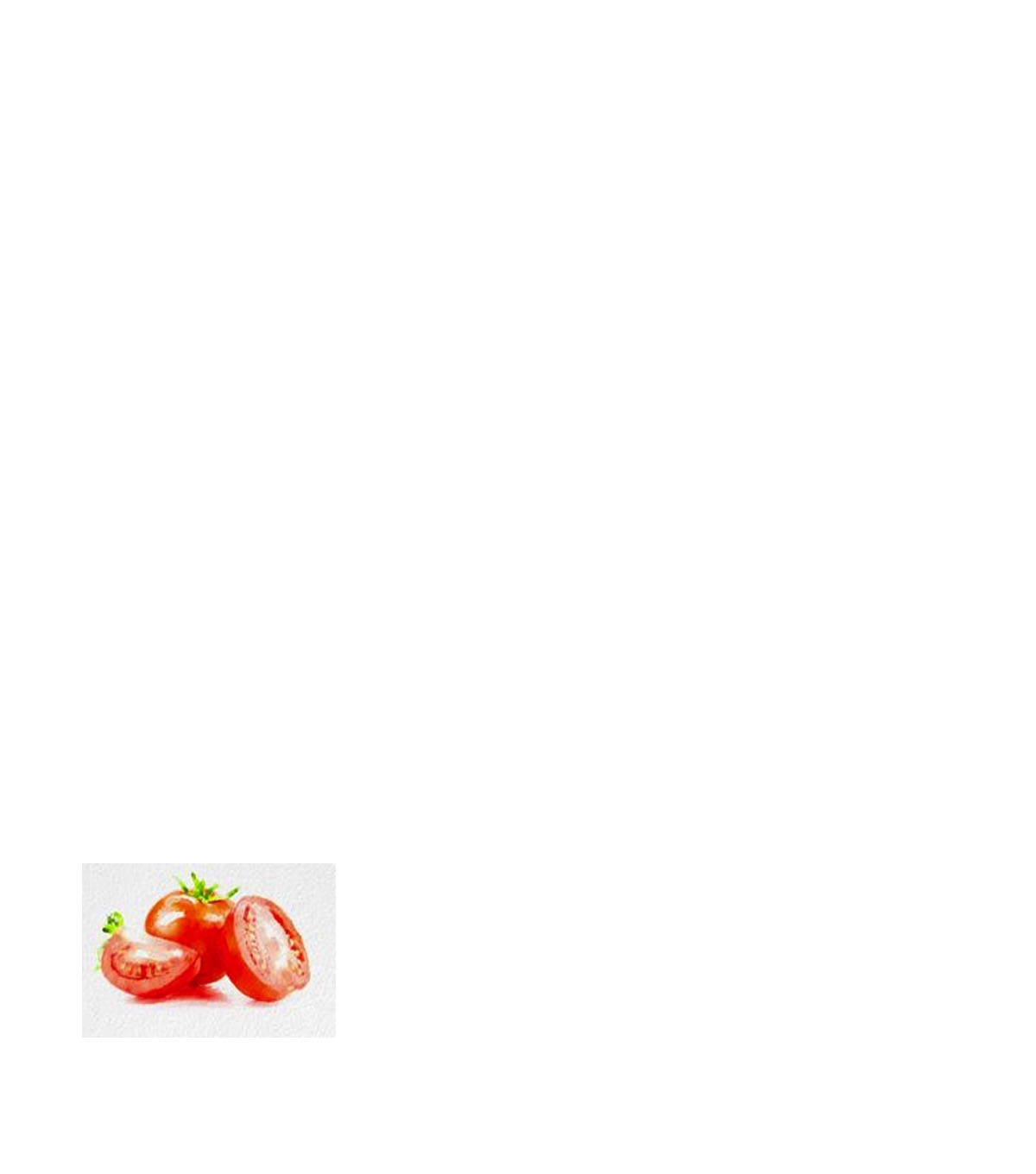
|
Original Image 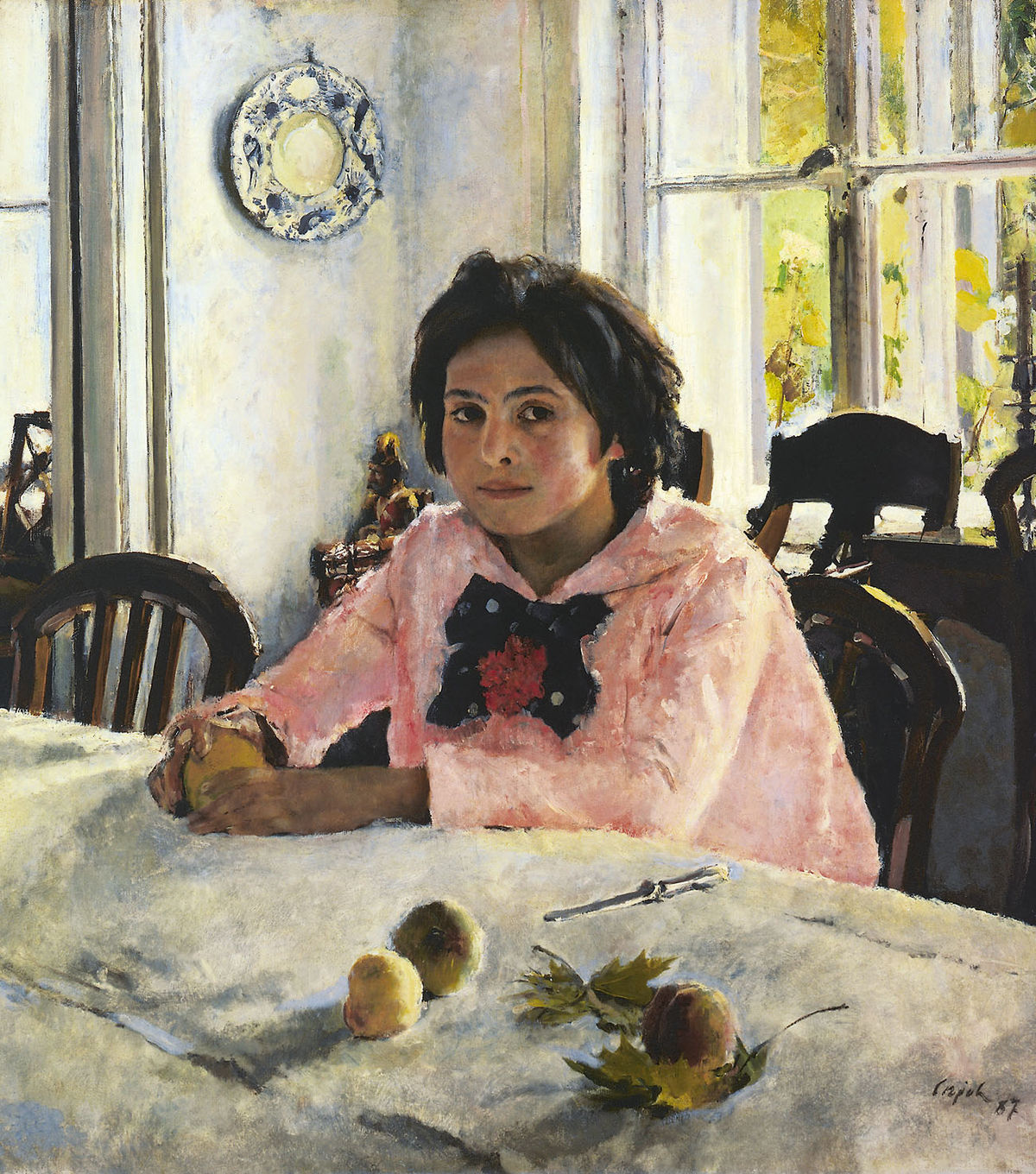
|
Mask 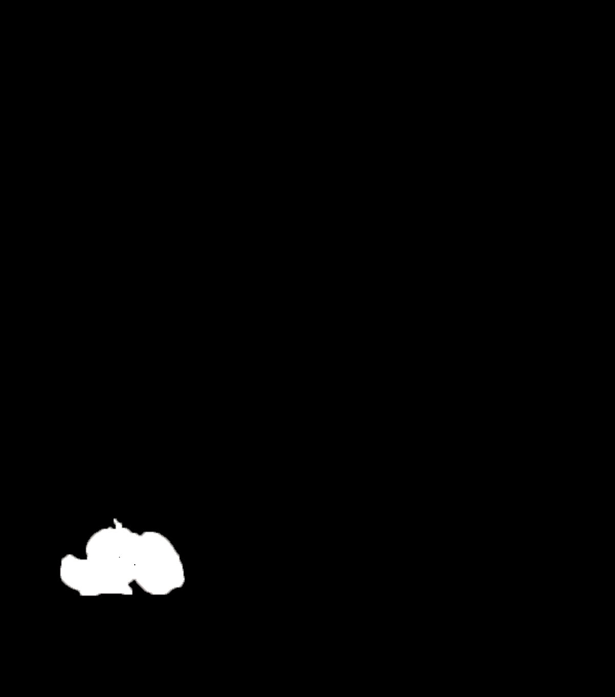
|
Blended 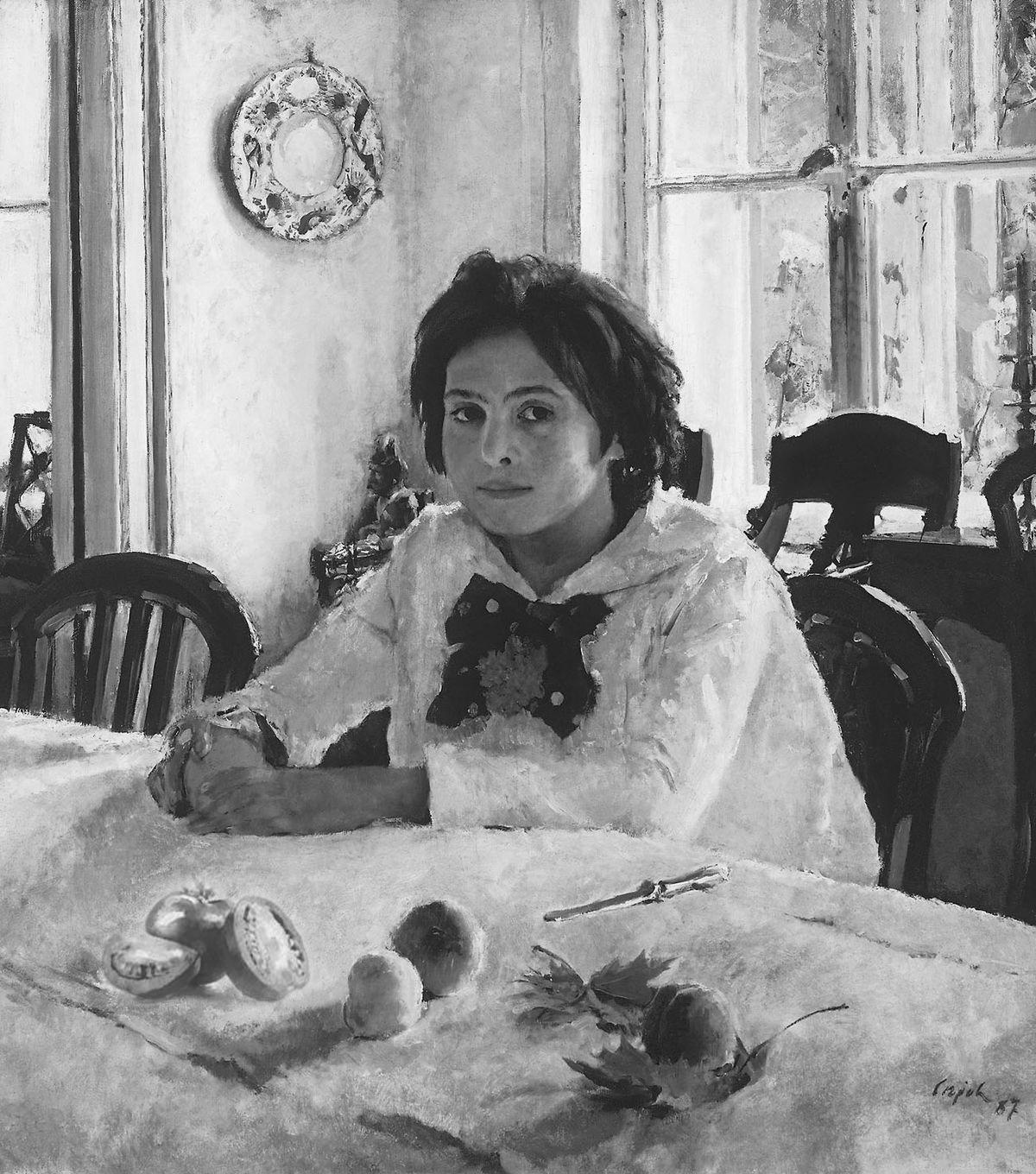
|
|
Original Image 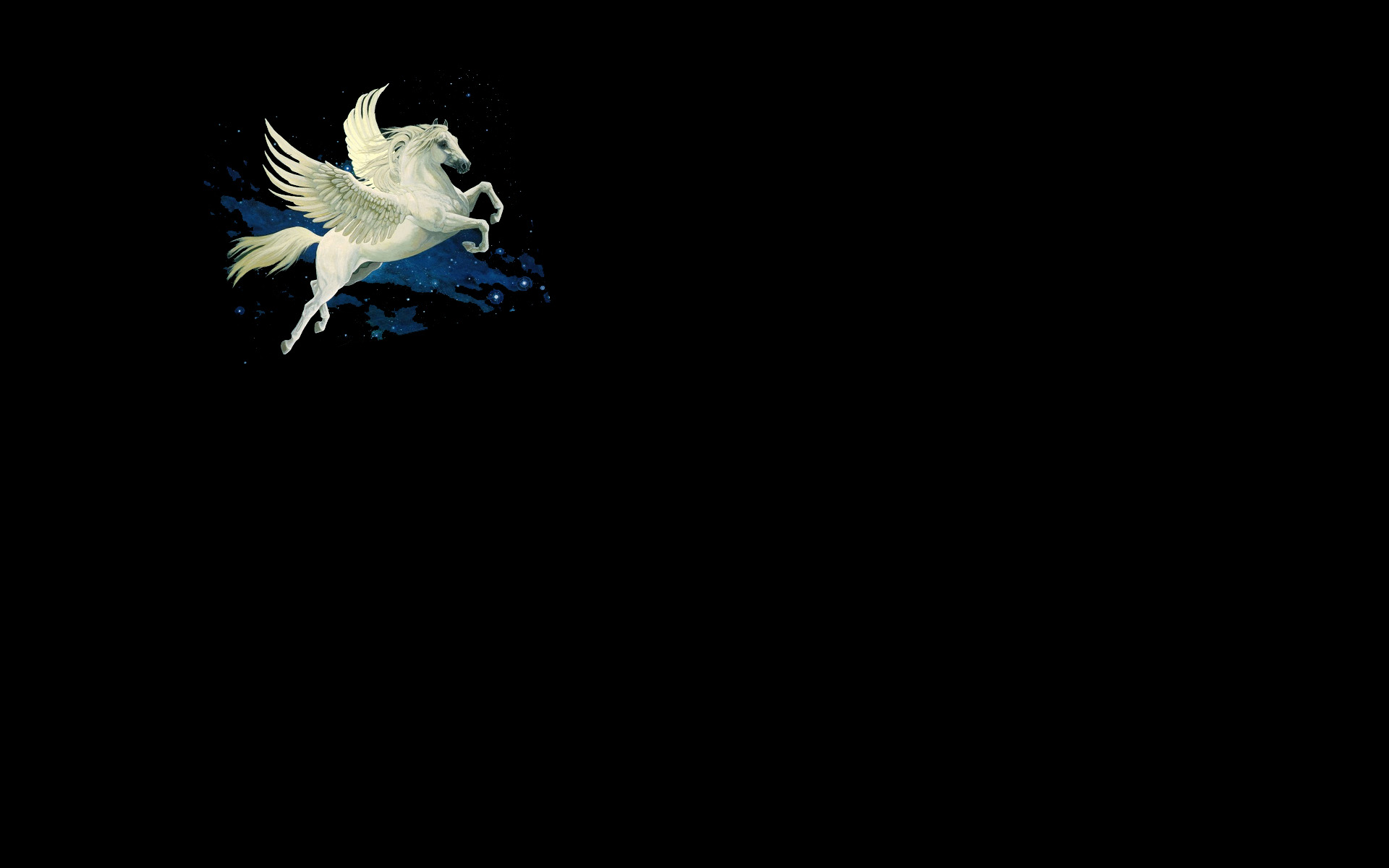
|
Original Image 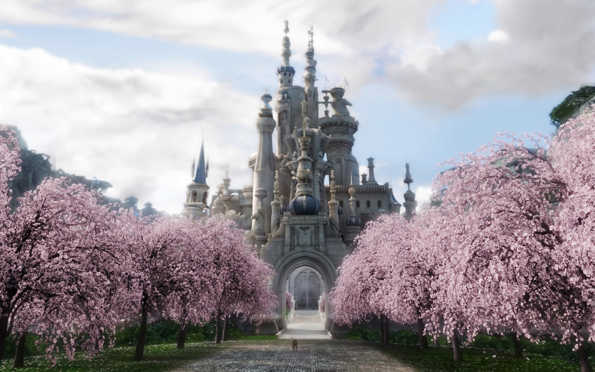
|
Mask 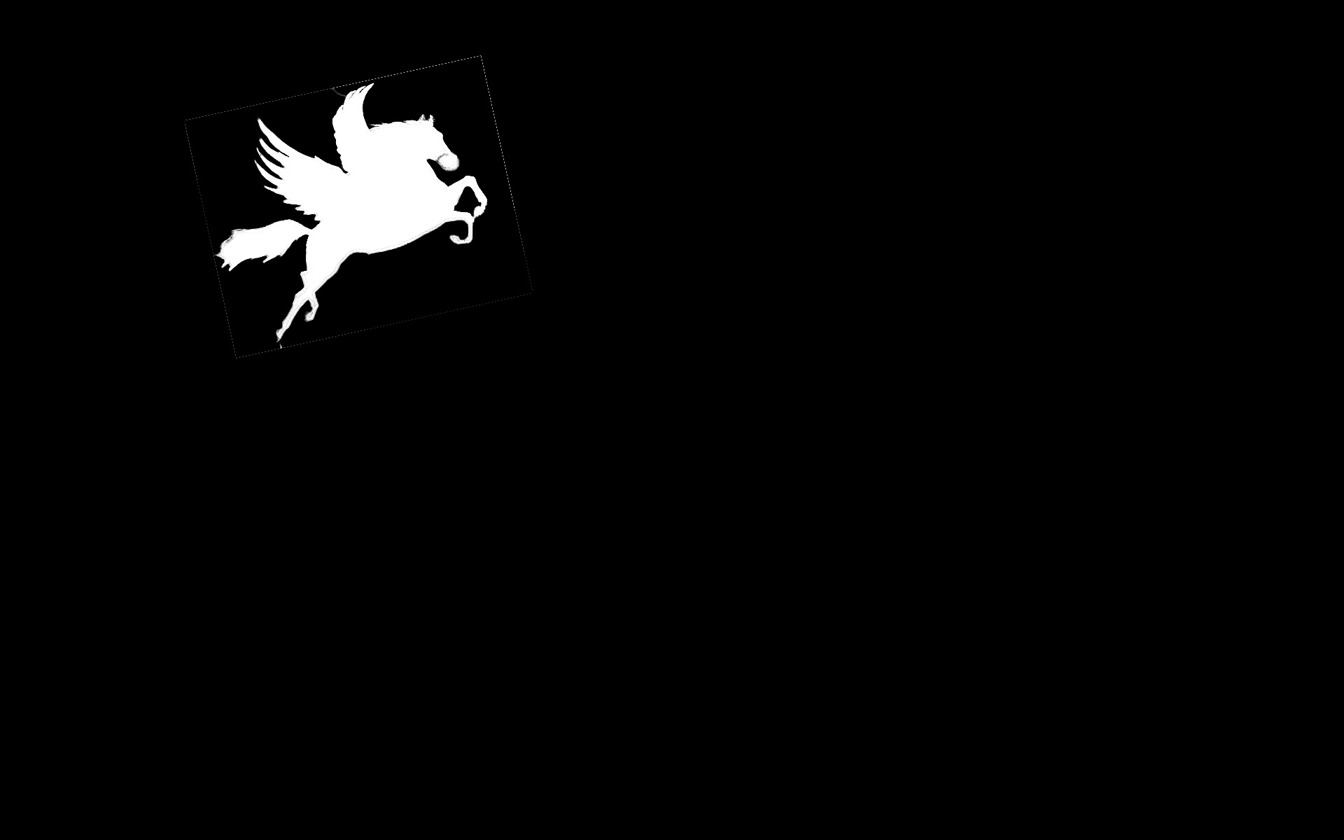
|
Blended 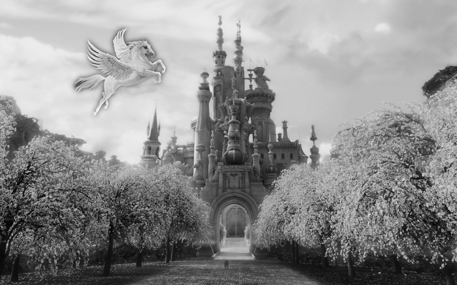
|
Colorized Images
|
Original Image
|
Original Image
|
Mask
|
Blended 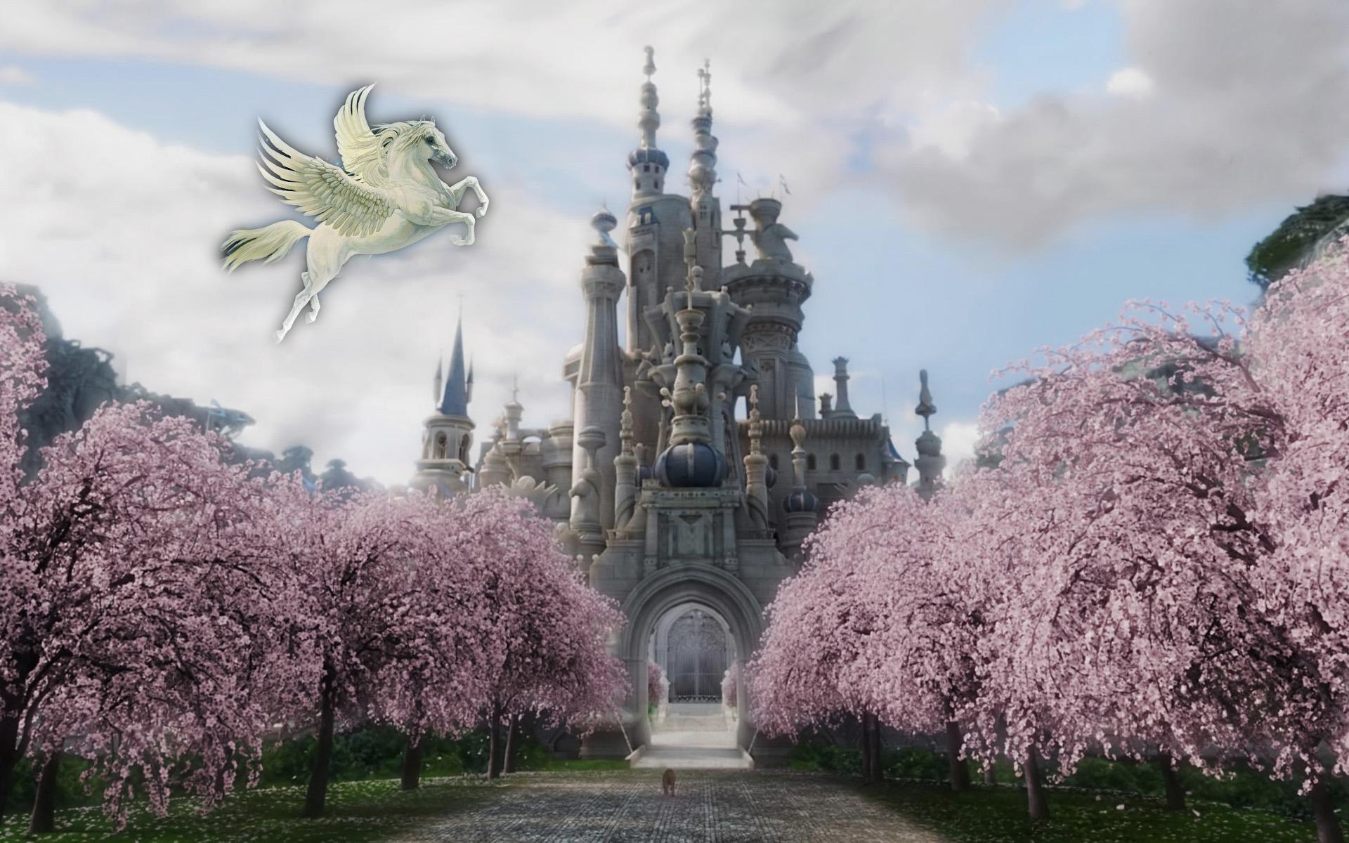
|
|
Original Image 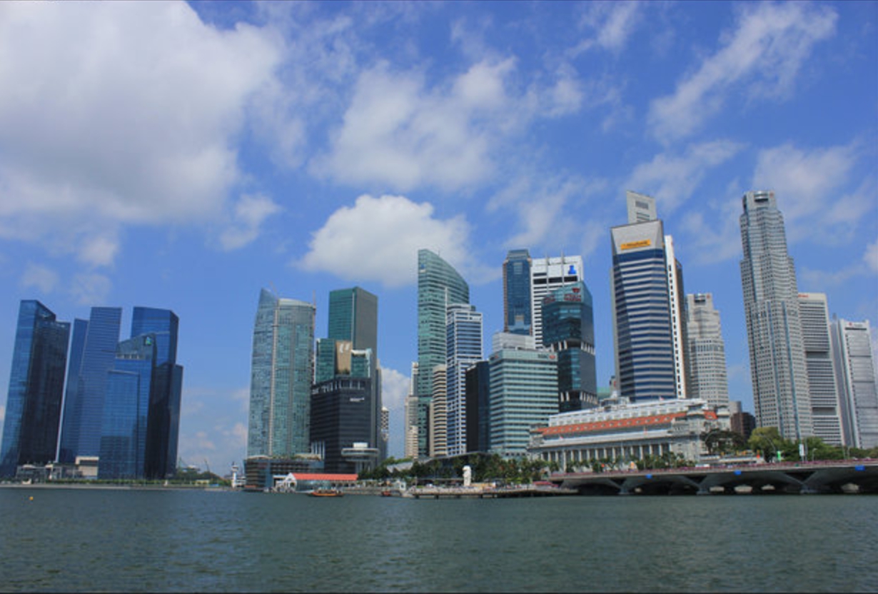
|
Original Image 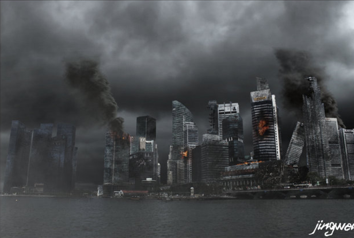
|
Mask 
|
Blended 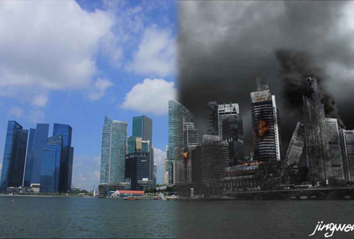
|
|
Original Image
|
Original Image
|
Mask
|
Blended 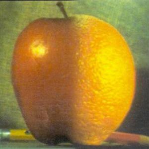
|
|
Original Image
|
Original Image
|
Mask
|
Blended 
|
Part 2: Gradient Domain Fusion
OverviewThe primary goal of this part of the project is to seamlessly blend an object into a target image, but instead of using Laplacian pyramid blending, we will use Poisson blending. As gradients play more important role than overall pixel intensity, Poisson blending finds pixel values so as to maximally preserve the gradient of source image. This way the objective function can be written as a least-squares problem. Given the pixel intensities of the source image "s" and target image "t", we want to solve for new intensity values "v" within the source region:

Poisson blending consists of the general idea to solve for specified pixels intensities and gradients in order to create a blended image. The newly constructed image "v" has its gradients inside the soure region that are similar to the gradients of image source image and the initial pixel intensities for the pixels on the borders of the mask are the same as those in image "t". For the rest of the pixels, we will just copy those from image "t" directly.
Part 2.1: Toy Problem
Results|
Original Image 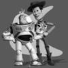
|
Recovered Image 
|
Part 2.2: Poisson Blending
Favorite Blending Result|
Source 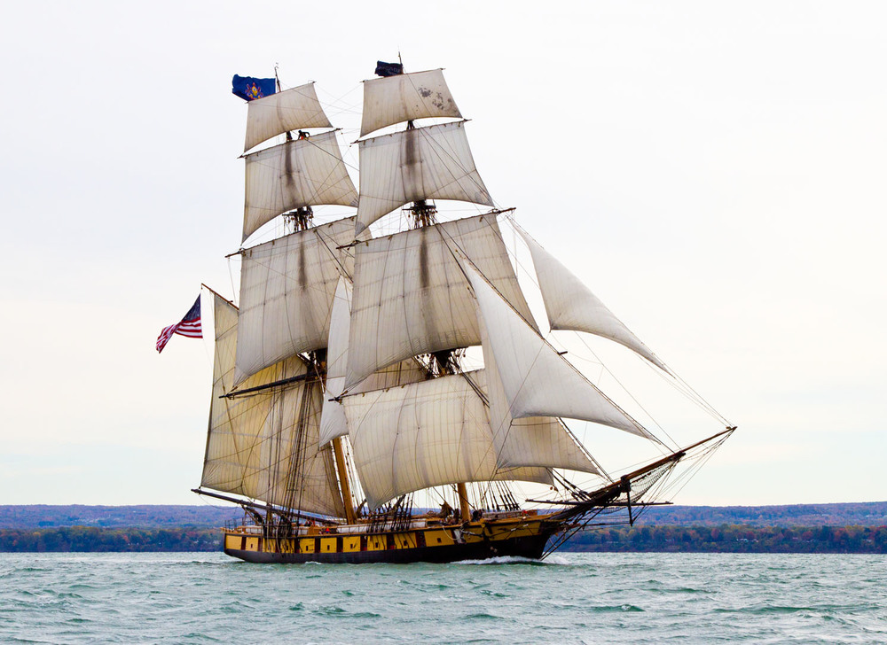
|
Target 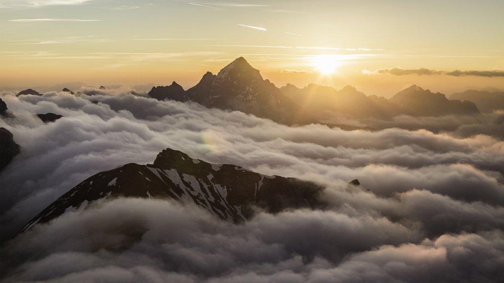
|
Directly Copied Pixels 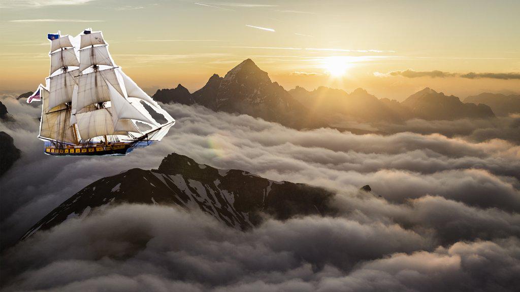
|
Poission Blended Image 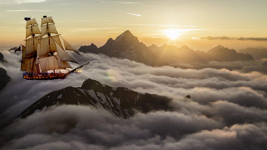
|
To get the Possion Blended image I analyzed all the pixels in a padded rectangle around the mask. I only take this pixels into consideration to improve runtime. First, I mapped each pixel in that area to an index. This is to keep track of every equation. I made a copy of the flattened target and saved it as a vector b. Then I populated a sparse matrix A according to the following logic: for each pixel_idx (pixel index) in the rectangle - if the pixel is in the mask, then calculate the gradient of that pixel at the source and set the value of b[pixel_idx] to that gradient. For the that pixel I also want to find its 4-neighbors and scale them by -1, while scaling the original pixel by 4. This means I am applying a Laplacian mask to the "variable" matrix. If the pixel_idx is not in the mask, I simply set the entry of A[pixel_idx, pixel_idx] = 1 to ensure that pixel has the same intensity as in the target image. Finally, I solve x = A/b. This gives the resulting x that needs to be reshaped and copied into the original target image.
|
Source 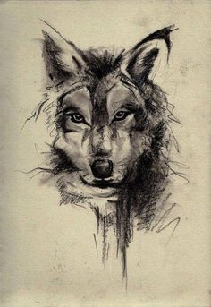
|
Target 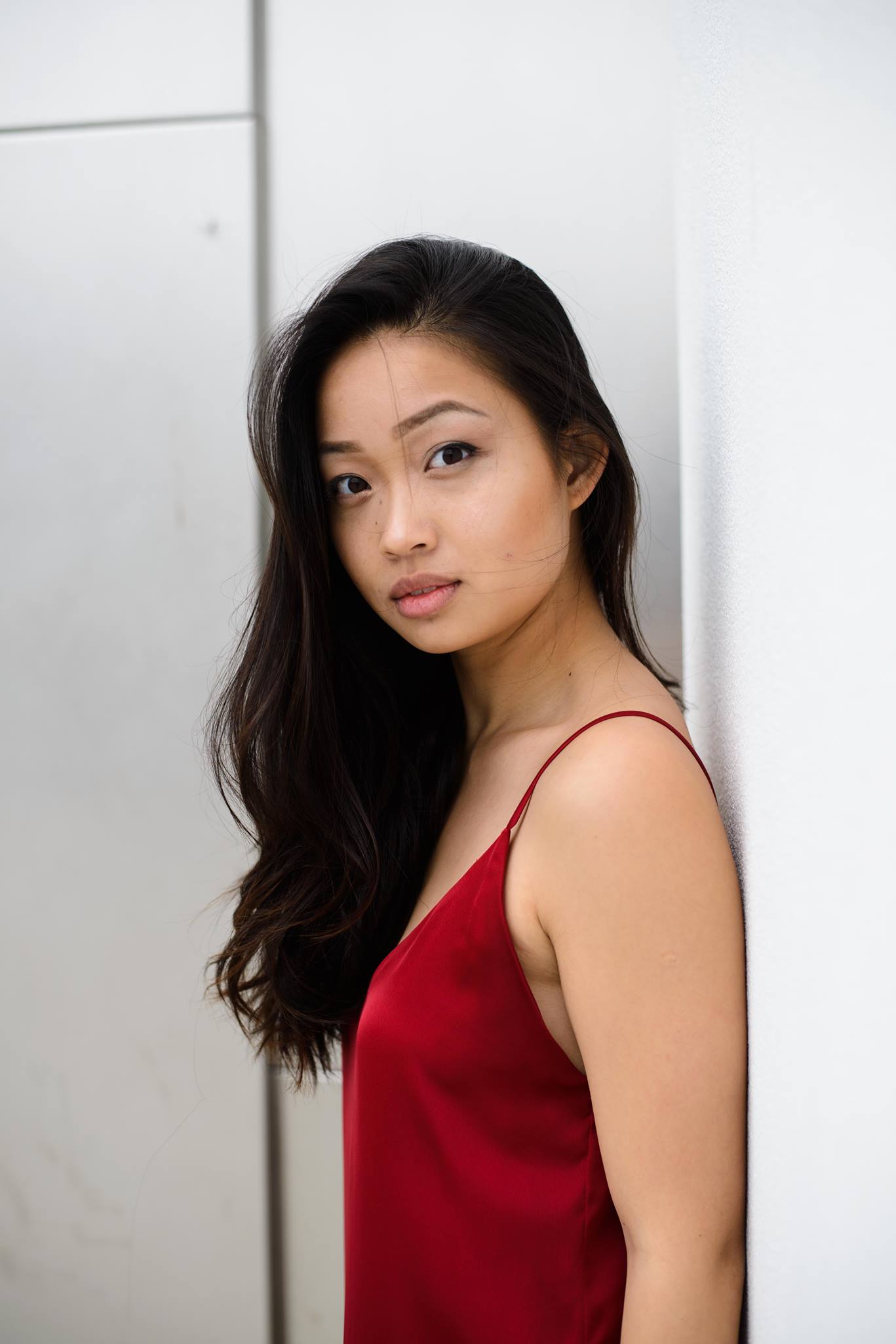
|
Directly Copied Pixels 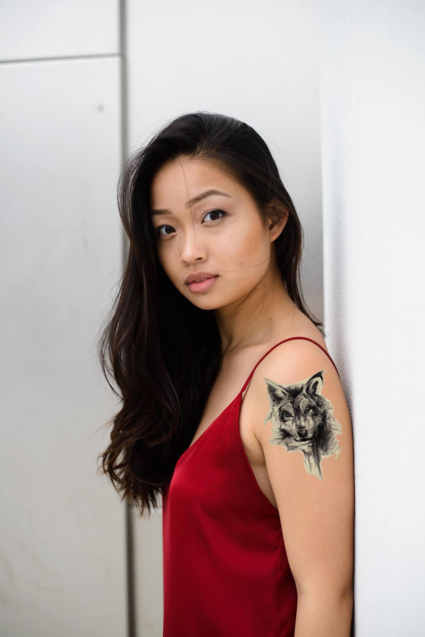
|
Poission Blended Image 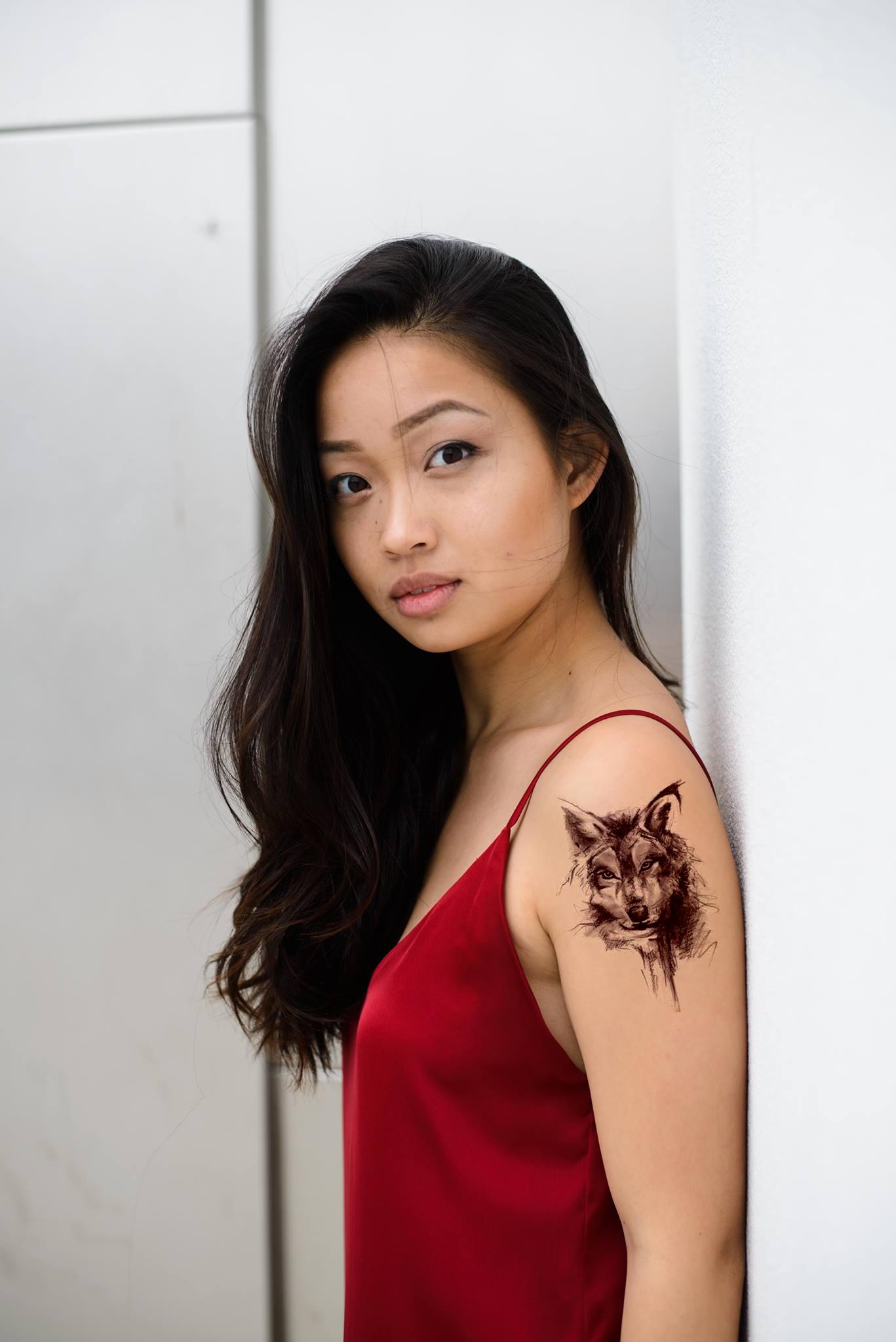
|
|
Source
|
Target 
|
Directly Copied Pixels 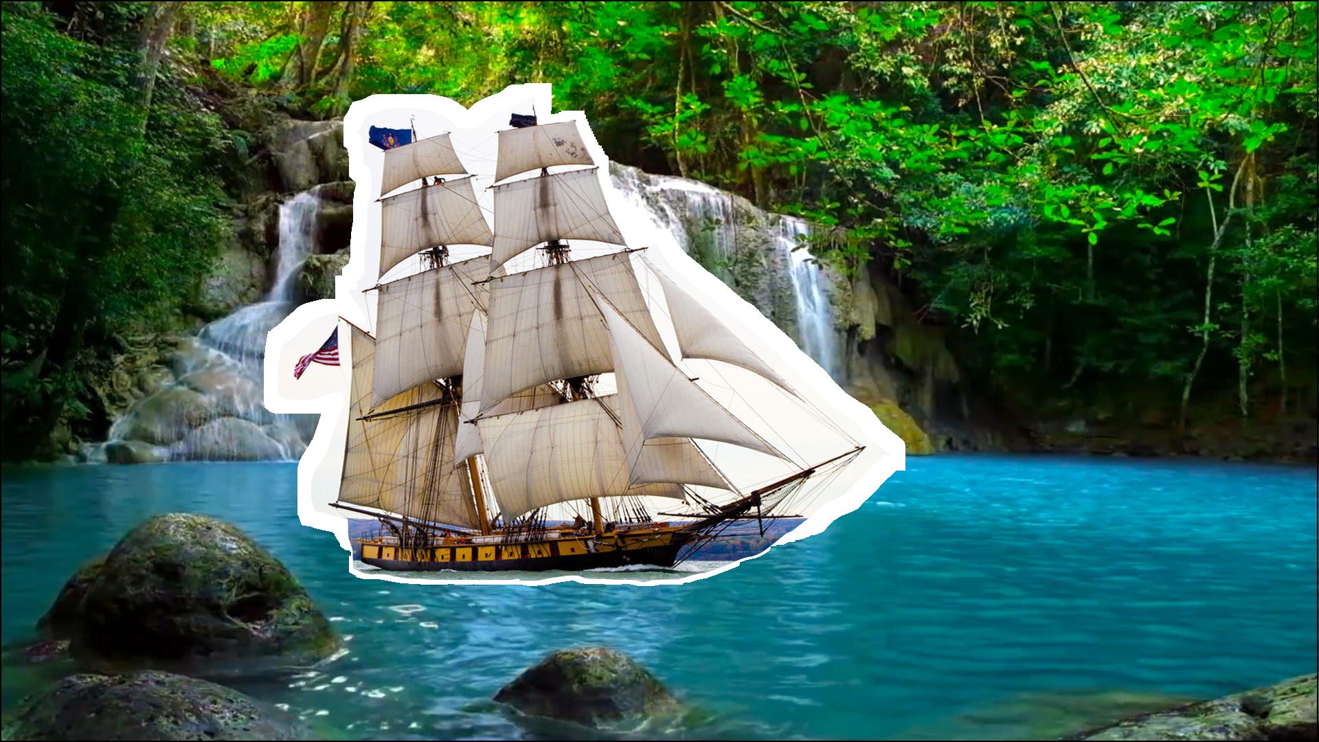
|
Poission Blended Image 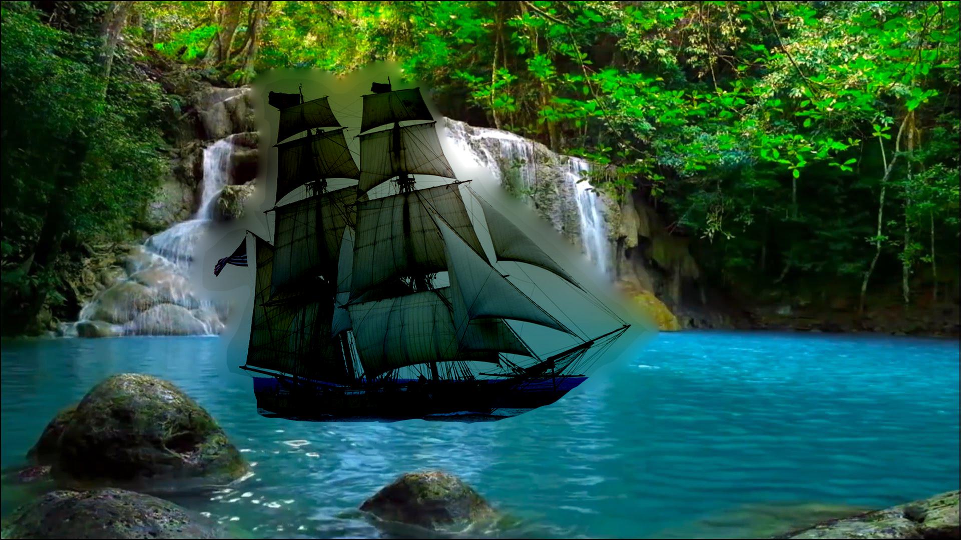
|
The reason this result of the Poisson Blending algorithm here is not aesthetically pleasing is because the background pixel values are not only too dark (compared to the pixel intesities of the source image) at some areas, but they also have an abrupt transition from light to dark in the middle. Because the algorthm approximates the border pixels to their neighbours, this color inconsistency is propagated onto the textures (gradients) of the source image.
Poisson Fusion VS Laplacian Stack Blending
|
Source 
|
Target 
|
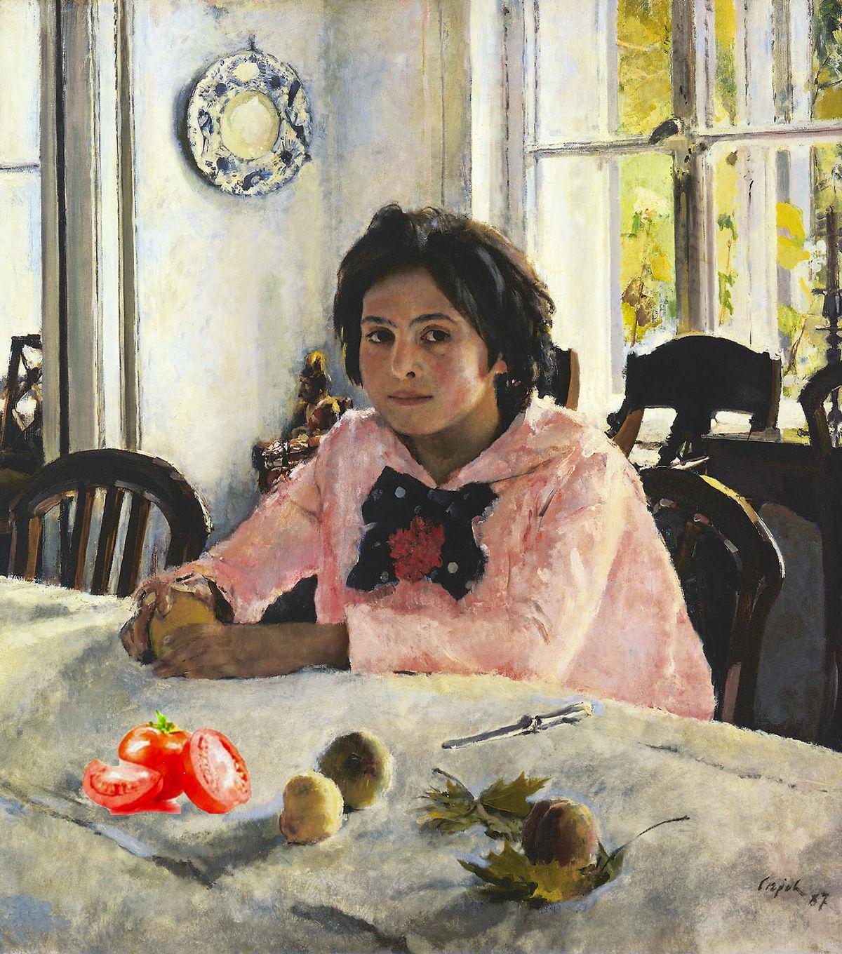
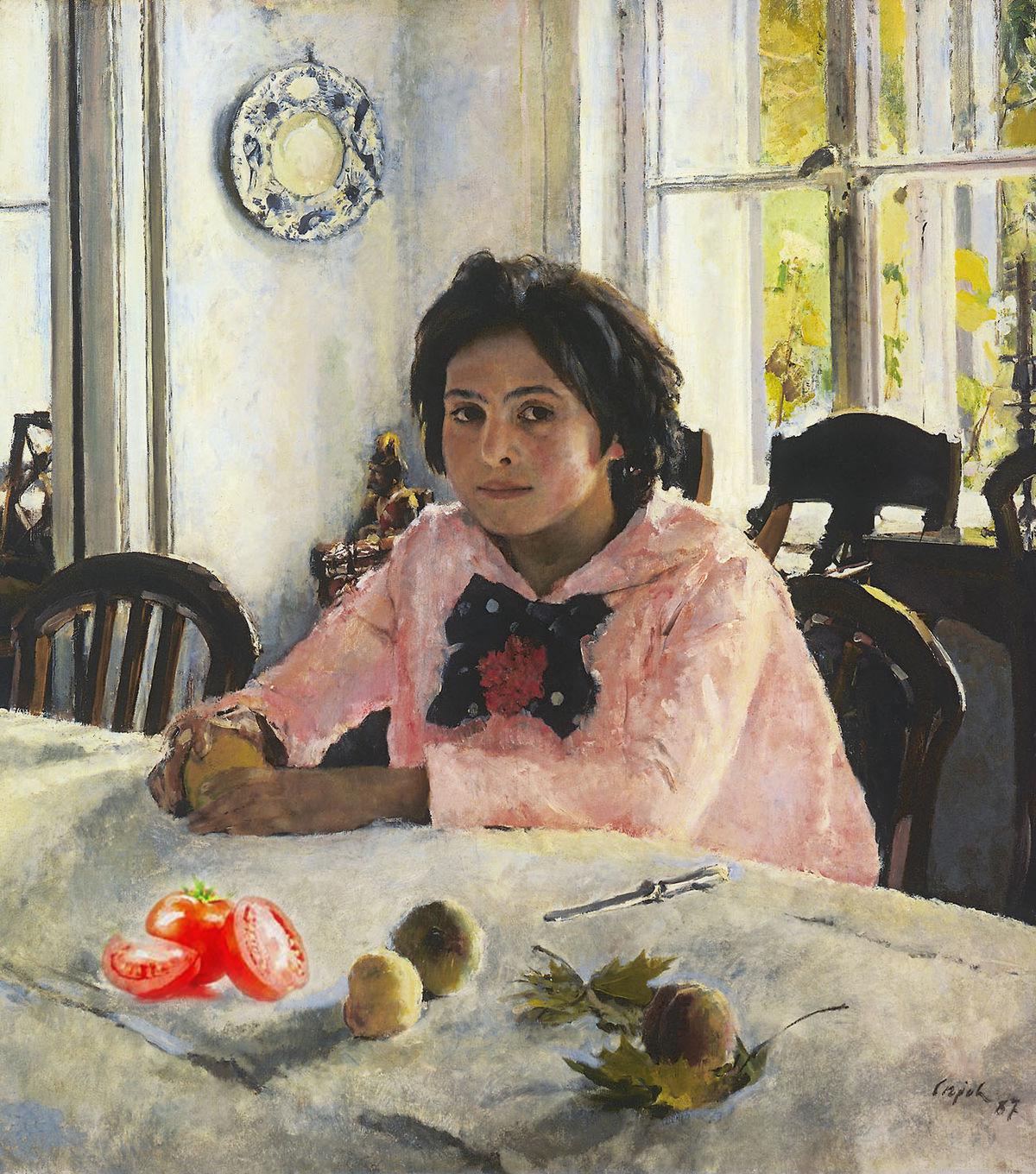

For the first image you can see the border of where the mask is defined between the source and the background image. Because the mask was generated pretty closely to the original source image, if you were to zoom out, you might not notice it, but it is still there.
The image constructed with a Laplacian Stack Blending solves the problem of easing out the edges between too images. You will notice, however, that the intensity of color remains the same for the source image. The background image is a famous work of art, composed in very distinct tones. And the bright red clipart tomato really clashes with the composition of the background.
Poisson Fusion solves all of the problems described about. Not only does it help get rid fo the edge between to images, it adjusts the pixel intensities of the source image to match those of the background image. The red color is toned down to make the addition of a tomato more appropriate for the compositon of the original art piece.